The LIFETEST Procedure

Life-Table Method
The life-table estimates are computed by counting the numbers of censored and uncensored observations that fall into each
of the time intervals  ,
,  , where
  and
and  . Let
. Let  be the number of units that enter the interval , and let
  be the number of events that occur in the interval. Let
  , and let
  , where
  is the number of units censored in the interval. The effective sample size of the interval is denoted by
  .
Let
.
Let  denote the midpoint of .
The conditional probability of an event in is estimated by
![\[ \hat{q}_ i = \frac{d_ i}{n_ i^{\prime }} \]](images/statug_lifetest0100.png)
and its estimated standard error is
![\[ \hat{\sigma } \left( \hat{q}_ i \right) = \sqrt { \frac{ \hat{q}_ i \hat{p}_ i }{ n_ i^{\prime } } } \]](images/statug_lifetest0101.png)
where  .
.
The estimate of the survival function at  is
is
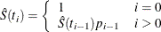
and its estimated standard error is
![\[ \hat{\sigma } \left( \hat{S}(t_ i) \right) = \hat{S}(t_ i) \sqrt { \sum _{j=1}^{i-1} \frac{ \hat{q}_ j }{ n_ j^{\prime } \hat{p}_ j } } \]](images/statug_lifetest0104.png)
The density function at is estimated by
![\[ \hat{f}(t_{mi}) = \frac{ \hat{S}(t_{i}) \hat{q}_ i }{b_ i} \]](images/statug_lifetest0105.png)
and its estimated standard error is
![\[ \hat{\sigma } \left( \hat{f}(t_{mi}) \right) = \hat{f}(t_{mi}) \sqrt { \sum _{j=1}^{i-1} \frac{ \hat{q}_ j }{ n_ j^{\prime } \hat{p}_ j } + \frac{ \hat{p}_ i }{ n_ i^{\prime } \hat{q}_ i } } \]](images/statug_lifetest0106.png)
The estimated hazard function at is
![\[ \hat{h}(t_{mi}) = \frac{ 2 \hat{q}_ i }{ b_ i(1 + \hat{p}_ i) } \]](images/statug_lifetest0107.png)
and its estimated standard error is
![\[ \hat{\sigma } \left( \hat{h}(t_{mi}) \right) = \hat{h}(t_{mi}) \sqrt { \frac{ 1 - ( b_ i \hat{h}(t_{mi})/2 )^2 }{ n_ i^{\prime } \hat{q}_ i } } \]](images/statug_lifetest0108.png)
Let  be the interval in which
  . The median residual lifetime at is estimated by
![\[ \hat{M}_ i = t_{j-1} - t_ i + b_ j \frac{ \hat{S}(t_{j-1}) - \hat{S}(t_ i)/2}{ \hat{S}(t_{j-1}) - \hat{S}(t_ j) } \]](images/statug_lifetest0111.png)
and the corresponding standard error is estimated by
![\[ \hat{\sigma }(\hat{M}_ i) = \frac{ \hat{S}(t_ i) }{ 2 \hat{f}(t_{mj}) \sqrt {n_ i^{\prime }} } \]](images/statug_lifetest0112.png)
Interval Determination
If you want to determine the intervals exactly, use the INTERVALS= option in the PROC LIFETEST statement to specify the interval
endpoints. Use the WIDTH= option to specify the width of the intervals, thus indirectly determining the number of intervals.
If neither the INTERVALS= option nor the WIDTH= option is specified in the life-table estimation, the number of intervals
is determined by the NINTERVAL= option. The width of the time intervals is 2, 5, or 10 times an integer (possibly a negative
integer) power of 10. Let  (maximum observed time/number of intervals), and let b be the largest integer not exceeding c. Let
  and let
![\[ a = 2 \times I(d \leq 2) + 5 \times I(2 < d \leq 5) + 10 \times I(d > 5) \]](images/statug_lifetest0115.png)
with I being the indicator function. The width is then given by
![\[ \mbox{width} = a \times 10^{b} \]](images/statug_lifetest0116.png)
By default, NINTERVAL=10.