The HPLMIXED Procedure

Estimating Covariance Parameters in the Mixed Model
Estimation is more difficult in the mixed model than in the general linear model. Not only do you have  as in the general linear model, but you also have unknown parameters in
  ,
,  , and
, and  . Least squares is no longer the best method. Generalized least squares (GLS) is more appropriate, minimizing
![\[ (\mb{y} - \mb{X}\bbeta )’\mb{V}^{-1}(\mb{y} - \mb{X}\bbeta ) \]](images/statug_hplmixed0185.png)
However, GLS requires knowledge of  and therefore knowledge of and . Lacking such information, one approach is to use an estimated GLS, in which you insert some reasonable estimate for into the minimization problem. The goal thus becomes finding a reasonable estimate of and .
In many situations, the best approach is to use likelihood-based methods, exploiting the assumption that and  are normally distributed (Hartley and Rao 1967; Patterson and Thompson 1971; Harville 1977; Laird and Ware 1982; Jennrich and Schluchter 1986). PROC HPLMIXED implements two likelihood-based methods: maximum likelihood (ML) and restricted (residual) maximum likelihood
(REML). A favorable theoretical property of ML and REML is that they accommodate data that are missing at random (Rubin 1976; Little 1995).
are normally distributed (Hartley and Rao 1967; Patterson and Thompson 1971; Harville 1977; Laird and Ware 1982; Jennrich and Schluchter 1986). PROC HPLMIXED implements two likelihood-based methods: maximum likelihood (ML) and restricted (residual) maximum likelihood
(REML). A favorable theoretical property of ML and REML is that they accommodate data that are missing at random (Rubin 1976; Little 1995).
PROC HPLMIXED constructs an objective function associated with ML or REML and maximizes it over all unknown parameters. Using
calculus, it is possible to reduce this maximization problem to one over only the parameters in and . The corresponding log-likelihood functions are as follows:
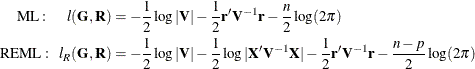
where  and p is the rank of
  . By default, PROC HPLMIXED actually minimizes a normalized form of
  times these functions by using a ridge-stabilized Newton-Raphson algorithm by default. Lindstrom and Bates (1988) provide reasons for preferring Newton-Raphson to the expectation-maximum (EM) algorithm described in Dempster, Laird, and
Rubin (1977) and Laird, Lange, and Stram (1987), in addition to analytical details for implementing a QR-decomposition approach to the problem. Wolfinger, Tobias, and Sall
(1994) present the sweep-based algorithms that are implemented in PROC HPLMIXED. You can change the optimization technique with
the TECHNIQUE=
option in the PROC HPLMIXED
statement.
times these functions by using a ridge-stabilized Newton-Raphson algorithm by default. Lindstrom and Bates (1988) provide reasons for preferring Newton-Raphson to the expectation-maximum (EM) algorithm described in Dempster, Laird, and
Rubin (1977) and Laird, Lange, and Stram (1987), in addition to analytical details for implementing a QR-decomposition approach to the problem. Wolfinger, Tobias, and Sall
(1994) present the sweep-based algorithms that are implemented in PROC HPLMIXED. You can change the optimization technique with
the TECHNIQUE=
option in the PROC HPLMIXED
statement.
One advantage of using the Newton-Raphson algorithm is that the second derivative matrix of the objective function evaluated
at the optima is available upon completion. Denoting this matrix  , the asymptotic theory of maximum likelihood (Serfling 1980) shows that
  is an asymptotic variance-covariance matrix of the estimated parameters of
  and
and  . Thus, tests and confidence intervals based on asymptotic normality can be obtained. However, these can be unreliable in
small samples, especially for parameters such as variance components that have sampling distributions that tend to be skewed
to the right.
. Thus, tests and confidence intervals based on asymptotic normality can be obtained. However, these can be unreliable in
small samples, especially for parameters such as variance components that have sampling distributions that tend to be skewed
to the right.
If a residual variance  is a part of your mixed model, it can usually be profiled out of the likelihood. This means solving analytically for the optimal and plugging this expression back into the likelihood formula (Wolfinger, Tobias, and Sall 1994). This reduces the number of optimization parameters by 1 and can improve convergence properties. PROC HPLMIXED profiles
the residual variance out of the log likelihood.
is a part of your mixed model, it can usually be profiled out of the likelihood. This means solving analytically for the optimal and plugging this expression back into the likelihood formula (Wolfinger, Tobias, and Sall 1994). This reduces the number of optimization parameters by 1 and can improve convergence properties. PROC HPLMIXED profiles
the residual variance out of the log likelihood.