The VARIOGRAM Procedure

This example helps you explore aspects of automated semivariogram fitting with PROC VARIOGRAM. The test case is a spatial study of arsenic (As) concentration in drinking water.
Arsenic is a toxic pollutant that can occur in drinking water because of human activity or, typically, due to natural release
from the sediments in water aquifers. The World Health Organization has a standard that allows As concentration up to a maximum of 10 ![]() g/lt (micrograms per liter) in drinking water.
g/lt (micrograms per liter) in drinking water.
In general, natural release of arsenic into groundwater is very slow. Arsenic concentration in water might exhibit no significant
temporal fluctuations over a period of a few months. For this reason, it is acceptable to perform a spatial study of arsenic
with input from time-aggregated pollutant concentrations. This example makes use of this assumption for its data set logAsData. The data set consists of 138 simulated observations from wells across a square area of 500 km ![]() 500 km. The variable
500 km. The variable logAs in the logAsData data set is the natural logarithm of arsenic concentration. Often, the natural logarithm of arsenic concentration (logAs) is used as the random variable to facilitate the analysis because its distribution tends to resemble the normal distribution.
The goal is to explore spatial continuity in the logAs observations. The following statements read the logAs values from the logAsData data set:
title 'Semivariogram Model Fitting of Log-Arsenic Concentration';

data logAsData;
   input East North logAs @@;
   label logAs='log(As) Concentration';
   datalines;
193.0 296.6 -0.68153   232.6 479.1  0.96279   268.7 312.5 -1.02908
 43.6   4.9  0.65010   152.6  54.9  1.87076   449.1 395.8  0.95932
310.9 493.6 -1.66208   287.8 164.9 -0.01779   330.0   8.0  2.06837
225.7 241.7  0.15899   452.3  83.4 -1.21217   156.5 462.5 -0.89031
 11.5  84.4 -0.24496   144.4 335.7  0.11950   149.0 431.8 -0.57251
234.3 123.2 -1.33642    37.8 197.8 -0.27624   183.1 173.9 -2.14558
149.3 426.7 -1.06506   434.4  67.5 -1.04657   439.6 237.0 -0.09074
 36.4 175.2 -1.21211   370.6 244.0  3.28091   452.0  96.5 -0.77081
247.0  86.8  0.04720   413.6 373.2  1.78235   253.5 291.7  0.56132
129.7 111.9  1.34000   352.7  42.1  0.23621   279.3  82.7  2.12350
382.6 290.7  0.86756   188.2 222.8 -1.23308   382.8 154.5 -0.94094
304.4 309.2 -1.95158   337.5 387.2 -1.31294   490.7 189.8  0.40206
159.0 100.1 -0.22272   245.5 329.2 -0.26082   372.1 379.5 -1.89078
417.8  84.1 -1.25176   173.9 407.6 -0.24240   121.5 107.7  1.54509
453.5 313.6  0.65895   143.5 346.7 -0.87196   157.4 125.5 -1.96165
371.8 353.2 -0.59464   358.9 338.2 -1.07133     8.6 437.8  1.44203
395.9 394.2 -0.24144   149.5  58.9  1.17459   453.5 420.6 -0.63951
182.3  85.0  1.00005    21.0 290.1  0.31016    11.1 352.2 -0.88418
131.2 238.4 -0.57184   104.9   6.3  1.12054   247.3 256.0  0.14019
428.4 383.7  0.92448   327.8 481.1 -2.72543   199.2  92.8 -0.05717
453.9 230.1  0.16571   205.0 250.6  0.07581   459.5 271.6  0.93700
229.5 262.8  1.83590   370.4 228.6  2.96611   330.2 281.9  1.79723
354.8 388.3 -3.18262   406.2 222.7  2.41594   254.4 393.1  2.03221
 96.7  85.2 -0.47156   407.2 256.8  0.66747   498.5 273.8  1.03041
417.2 471.4 -1.42766   368.8 424.3 -0.70506   303.0  59.1  1.43070
403.1 264.1  1.64554    21.2 360.8  0.67094   148.2  78.1  2.15323
305.5 310.7 -1.47985   228.5 180.3 -0.68386   161.1 143.3  1.07901
 70.5 155.1  0.54652   363.1 282.6 -0.43051    86.0 472.5 -1.18855
175.9 105.3 -2.08112    96.8 426.3  1.56592   475.1 453.1 -1.53776
125.7 485.4  1.40054   277.9 201.6 -0.54565   406.2 125.0 -1.38657
 60.0 275.5 -0.59966   431.3 494.6 -0.36860   399.9 399.0 -0.77265
 28.8 311.1  0.91693   166.1 348.2 -0.49056   266.6  83.5  0.67277
 54.7 356.3  0.49596   433.5 460.3 -1.61309   201.7 167.6 -1.40678
158.1 203.6 -1.32499    67.6 230.4  1.14672    81.9 250.0  0.63378
372.0  50.7  0.72445    26.4 264.6  1.00862   300.1  91.7 -0.74089
303.0 447.4  1.74589   108.4 386.2  1.12847    55.6 191.7  0.95175
 36.3 273.2  1.78880    94.5 298.3 -2.43320   366.1 187.3 -0.80526
130.7 389.2 -0.31513    37.2 324.2  0.24489   295.5 211.8  0.41899
 58.6 206.2  0.18495   346.3 142.8 -0.92038   484.2 215.9  0.08012
451.4 415.7  0.02773    58.9  86.5  0.17652   212.6 363.9  0.17215
378.7 407.6  0.51516   265.9 305.0 -0.30718   123.2 314.8 -0.90591
 26.9 471.7  1.70285    16.5   7.1  0.51736   255.1 472.6  2.02381
111.5 148.4 -0.09658   440.4 375.0  1.23285   406.4  19.5  1.01181
321.2  65.8 -0.02095   466.4 357.1 -0.49272     2.0 484.6  0.50994
200.9 205.1  0.43543    30.3 337.0  1.60882   297.0  12.7  1.79824
158.2 450.7  0.05295   122.8 105.3  1.53936   417.8 329.7 -2.08124
;
First you want to inspect the logAs data for surface trends and the pairwise distribution. You run the VARIOGRAM procedure with the NOVARIOGRAM option in the COMPUTE statement. You also request the PLOTS=PAIRS(MID) option, which prompts the pair distance plot to display the actual distance between pairs, rather than the lag number itself, in the midpoint of the lags. You use the following statements:
ods graphics on;
proc variogram data=logAsData plots=pairs(mid);
   compute novariogram nhc=50;
   coord xc=East yc=North;
   var logAs;
run;
The observations scatter plot in Output 109.1.1 shows a rather uniform distribution of the locations in the study domain. Reasonably, neighboring values of logAs seem to exhibit some correlation. There seems to be no definite sign of an overall surface trend in the logAs values. You can consider that the observations are trend-free, and proceed with estimation of the empirical semivariance.
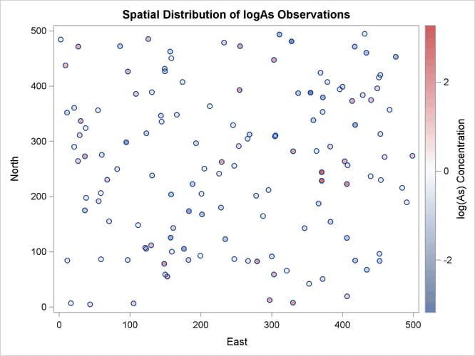
The observed logAs values go as high as 3.28091, which corresponds to a concentration of 26.6 ![]() g/lt. In fact, only three observations exceed the health standard of 10
g/lt. In fact, only three observations exceed the health standard of 10 ![]() g/lt (or about 2.3 in the log scale), and they are situated in relatively neighboring locations to the east of the domain
center.
g/lt (or about 2.3 in the log scale), and they are situated in relatively neighboring locations to the east of the domain
center.
Based on the discussion in section Preliminary Spatial Data Analysis, the pair distance plot in Output 109.1.2 suggests that you could consider pairs that are anywhere around up to half the maximum pairwise distance of about 700 km.
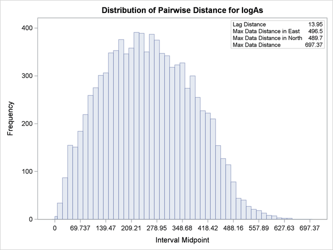
After some experimentation with values for the LAGDISTANCE=
and MAXLAGS=
options, you actually find that a lag distance of 5 km over 40 lags can provide a clear representation of the logAs semivariance. With respect to Output 109.1.2, this finding indicates that in the current example it is sufficient to consider pairs separated by a distance of up to 200
km. You run the following statements to obtain the empirical semivariogram:
proc variogram data=logAsData plots(only)=semivar;
   compute lagd=5 maxlag=40;
   coord xc=East yc=North;
   var logAs;
run;
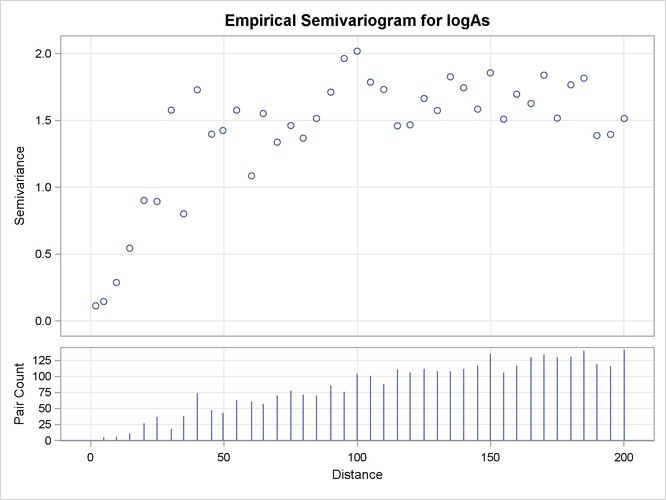
The first few lag classes of the logAs empirical semivariance table are shown in Output 109.1.3.
Output 109.1.3 and Output 109.1.4 indicate that the logarithm of arsenic spatial correlation starts with a small nugget effect around 0.11 and rises to a sill
value that is most likely between 1.4 and 1.8. The rise could be of exponential type, although the smooth increase of semivariance
close to the origin could also suggest Gaussian behavior. You suspect that a Matérn form might also work, since its smoothness
parameter ![]() can regulate the form to exhibit an intermediate behavior between the exponential and Gaussian forms.
can regulate the form to exhibit an intermediate behavior between the exponential and Gaussian forms.
You can investigate all of the preceding clues with the model fitting features of PROC VARIOGRAM. The simplest way to fit
a model is to specify its form in the MODEL
statement. In this case, you have the added complexity of having more than one possible candidate. For this reason, you use
the FORM=AUTO
option that picks the best fit out of a list of candidates. Within this option you specify the MLIST=
suboption to use the exponential, Gaussian, and Matérn forms. You also specify the NEST=
suboption to request fitting of a model with up to two nested structures. Eventually, you specify the PLOTS=FIT
option to produce a plot of the fitted models. The STORE
statement saves the fitting output into an item store you name SemivAsStore for future use. You apply these specifications with the following statements:
proc variogram data=logAsData plots(only)=fit;
   store out=SemivAsStore / label='LogAs Concentration Models';
   compute lagd=5 maxlag=40;
   coord xc=East yc=North;
   model form=auto(mlist=(exp,gau,mat) nest=1 to 2);
   var logAs;
run;

ods graphics off;
The table of general information about fitting is shown in Output 109.1.5. The table lets you know that 12 model combinations are to be tested for weighted least squares fitting, based on the three forms that you specified.
The combinations include repetitions. For example, you specified the GAU form; hence the GAU-GAU form is tested, too. The
model combinations also include permutations. For example, you specified the GAU and the EXP forms; hence the GAU-EXP and
EXP-GAU models are fitted separately. According to the section Nested Models, it might seem that the same model is fitted twice. However, in each of these two cases, each structure starts the fitting
process with different parameter initial values. This can lead GAU-EXP to a different fit than EXP-GAU leads to, as seen in
the fitting summary table in Output 109.1.6. The table shows all the model combinations that were tested and fitted. By default, the ordering is based on the weighted
sum of squares error criterion, and you can see that the lowest values in the Weighted SSE column are in top slots of the list.
Output 109.1.6: Semivariogram Model Fitting Summary
| Fit Summary | |||
|---|---|---|---|
| Class | Model | Weighted SSE |
AIC |
| 1 | Gau-Gau | 25.42435 | -9.59246 |
| Gau-Mat | 25.42482 | -7.59169 | |
| 2 | Exp-Gau | 25.97835 | -8.70865 |
| 3 | Exp-Mat | 26.36846 | -6.09754 |
| 4 | Mat | 26.37519 | -10.08708 |
| 5 | Gau | 26.78629 | -11.45296 |
| 6 | Exp | 28.01200 | -9.61851 |
| Exp-Exp | 28.01200 | -5.61850 | |
| Mat-Exp | 28.01200 | -3.61850 | |
| Gau-Exp | 28.01200 | -5.61850 | |
Note the leftmost Class column in Output 109.1.6. As explained in detail in section Classes of Equivalence, when you fit more than one model, all fitted models that compute the same semivariance are placed in the same class of equivalence.
For example, in this fitting example the top ranked GAU-GAU and GAU-MAT nested models produce indistinguishable semivariograms;
for that reason they are both placed in the same class 1 of equivalence. The same occurs with the EXP, GAU-EXP, EXP-EXP, and
MAT-EXP models in the bottom of the table. By default, PROC VARIOGRAM uses the AIC as a secondary classification criterion;
hence models in each equivalence class are already ordered based on their AIC values.
Another remark in Output 109.1.6 is that despite submitting 12 model combinations for fitting, the table shows only 10. You can easily see that the combinations
MAT-GAU and MAT-MAT are not among the listed models in the fit summary. This results from the behavior of the VARIOGRAM procedure
in the following situation: A parameter optimization takes place during the fitting process. In the present case the optimizer
keeps increasing the Matérn smoothness parameter ![]() in the MAT-GAU model. At the limit of an infinite
in the MAT-GAU model. At the limit of an infinite ![]() parameter, the Matérn form becomes the Gaussian form. For that reason, when the parameter
parameter, the Matérn form becomes the Gaussian form. For that reason, when the parameter ![]() is driven towards very high values, PROC VARIOGRAM automatically replaces the Matérn form with the Gaussian. This switch
converts the MAT-GAU model into a GAU-GAU model. However, a GAU-GAU model already exists among the specified forms; consequently,
the duplicate GAU-GAU model is skipped, and the fitted model list is reduced by one model. A similar explanation justifies
the omission of the MAT-MAT model from the fit summary table.
is driven towards very high values, PROC VARIOGRAM automatically replaces the Matérn form with the Gaussian. This switch
converts the MAT-GAU model into a GAU-GAU model. However, a GAU-GAU model already exists among the specified forms; consequently,
the duplicate GAU-GAU model is skipped, and the fitted model list is reduced by one model. A similar explanation justifies
the omission of the MAT-MAT model from the fit summary table.
In our example, the nested Gaussian-Gaussian model is the fitting selection of the procedure based on the default ranking criteria. Output 109.1.7 displays additional information about the selected model. In particular, you see the table with general information about the Gaussian-Gaussian model, the initial values used for its parameters, and information about the optimization process for the fitting.
The estimated parameter values of the selected Gaussian-Gaussian model are shown in Output 109.1.8.
By default, when you specify more than one model to fit, PROC VARIOGRAM produces a fit plot that compares the first five classes of the successfully fit candidate models. The model that is selected according to the specified fitting criteria is shown with a thicker line in the plot.
You can modify the number of displayed equivalence classes with the NCLASSES= suboption of the PLOTS=FIT option. When you have such comparison plots, PROC VARIOGRAM displays the representative model from each class of equivalence.
The default fit plot for the current model comparison is shown in Output 109.1.9. The legend informs you there is one more model in the first class of equivalence, as the fitting summary table indicated earlier in Output 109.1.6.
Output 109.1.9: Fitted Theoretical and Empirical logAs Concentration Semivariograms for the Specified Models
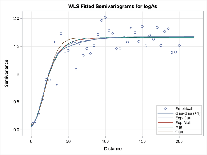
In the present example, all fitted models in the first five classes have very similar semivariograms. The selected Gaussian-Gaussian model seems to have a relatively larger range than the rest of the displayed models, but you can expect any of these models to exhibit a near-identical behavior in terms of spatial correlation. As a result, all models in the displayed classes are likely to lead to very similar output, if you proceed to use any of them for spatial prediction.
In that sense, semivariogram fitting is a partially subjective process, for which there might not exist only one single correct answer to solve your problem. In the context of the example, on one hand you might conclude that the selected Gaussian-Gaussian model is exactly sufficient to describe spatial correlation in the arsenic study. On the other hand, the similar performance of all models might prompt you to choose instead a more simple non-nested model for prediction like the Matérn or the Gaussian model.
Regardless of whether you might opt to sacrifice the statistically best fit (depending on your selected criteria) to simplicity, eventually you are the one to decide which approach serves your study optimally. The model fitting features of PROC VARIOGRAM offer you significant assistance so that you can assess your options efficiently.