The ROBUSTREG Procedure

The ROBUSTREG procedure uses the robust multivariate location and scatter estimates for leverage-point detection. The procedure computes a robust version of the Mahalanobis distance by using a generalized minimum covariance determinant (MCD) method. The original MCD method was proposed by Rousseeuw (1984).
PROC ROBUSTREG implements a generalized MCD algorithm that is based on the fast-MCD algorithm formulated by Rousseeuw and Van Driessen (1999), which is similar to the algorithm for least trimmed squares (LTS).
The canonical Mahalanobis distance is defined as
where ![]() and
and ![]() are the empirical multivariate location and scatter, respectively. Here
are the empirical multivariate location and scatter, respectively. Here ![]() excludes the intercept. The relationship between the Mahalanobis distance
excludes the intercept. The relationship between the Mahalanobis distance ![]() and the hat matrix
and the hat matrix ![]() is
is
The canonical robust distance is defined as
where ![]() and
and ![]() are the robust multivariate location and scatter, respectively, that are obtained by the MCD method.
are the robust multivariate location and scatter, respectively, that are obtained by the MCD method.
To achieve robustness, the MCD algorithm estimates the covariance of a multivariate data set mainly through an MCD h-point subset of the data set. This subset has the smallest sample-covariance determinant among all possible h-subsets. Accordingly, the breakdown value for the MCD algorithm equals ![]() . This means the MCD estimate is reliable, even if up to
. This means the MCD estimate is reliable, even if up to ![]() observations in the data set are contaminated.
observations in the data set are contaminated.
It is possible that the original data are in p-dimensional space but the h-point subset that yields the minimum covariance determinant lies in a lower-dimensional hyperplane. Applying the canonical MCD algorithm to such a data set would result in a singular covariance problem (called exact fit in Rousseeuw and Van Driessen 1999), such that the relevant robust distances cannot be computed. To deal with the singularity problem and provide further leverage-point analysis, PROC ROBUSTREG implements a generalized MCD algorithm. (For more information, see the section Generalized MCD Algorithm.) The algorithm distinguishes in-(hyper)plane points from off-(hyper)plane points, and performs MCD leverage-point analysis in the dimension-reduced space by projecting all points onto the hyperplane.
Low-dimensional structure is often induced by classification covariates. Suppose that, in a study that has 25 female subjects
and 5 male subjects, gender is the only classification effect. If the breakdown setting is greater than ![]() , the canonical MCD algorithm fails, and so does the relevant leverage-point analysis. In this case, the MCD h-subset would contain only female observations, and the constant gender in the h-subset would cause the relevant MCD estimate to be singular. The generalized MCD algorithm solves that problem by identifying
all male observations as off-plane leverage points, and then carries out the leverage-point analysis, with all the other covariates
being centered separately for female and male groups against their group means.
, the canonical MCD algorithm fails, and so does the relevant leverage-point analysis. In this case, the MCD h-subset would contain only female observations, and the constant gender in the h-subset would cause the relevant MCD estimate to be singular. The generalized MCD algorithm solves that problem by identifying
all male observations as off-plane leverage points, and then carries out the leverage-point analysis, with all the other covariates
being centered separately for female and male groups against their group means.
In general, low-dimensional structure is not necessarily due to classification covariates. Imagine that 80 children are supposed
to play on a straight trail (denoted by ![]() ) but that some adventurous children go off the trail. The following statements generate the
) but that some adventurous children go off the trail. The following statements generate the Children data set and the relevant scatter plot:
data Children;
   do i=1 to 80;
      off_trail=ranuni(321)>.9;
      x=rannor(111)*ranuni(321);
      trail_x=(i-40)/80*3;
      trail_y=trail_x;
      if off_trail=1 then y=x-1+rannor(321);
      else y=x;
      output;
   end;
run;
proc sgplot data=Children;
   series   x=trail_x y=trail_y/lineattrs=(color="red" pattern=4);
   scatter  x=x y=y/group=off_trail;
   ellipse  x=x y=y/alpha=.05 lineattrs=(color="green" pattern=34);
run;
Figure 86.17 shows the positions of all 80 children, the trail (as a red dashed line), and a contour curve of regular Mahalanobis distance
that is centered at the mean position (as a green dotted ellipse). In terms of regular Mahalanobis distance, the associated
covariance estimate is not singular, but its relevant leverage-point analysis completely ignores the trail (which is the entity
of the low-dimensional structure). The children outside the ellipse are defined as leverage points, but the children off the
trail would not be viewed as leverage points unless they had large Mahalanobis distances. As mentioned in Rousseeuw and Van Driessen
(1999), the canonical MCD method can find the low-dimensional structure, but it does not provide further robust covariance estimation
because the MCD covariance estimate is singular. As an improved version of the canonical MCD method, the generalized MCD method
can find the trail, identify the children off the trail as off-plane leverage points, and further execute in-plane leverage
analysis. The following statements apply the generalized MCD algorithm to the Children data set:
ods graphics on;
proc robustreg data=children plots=ddplot(label=none);
   model i = x y/leverage(mcdinfo opc);
run;
ods graphics off;
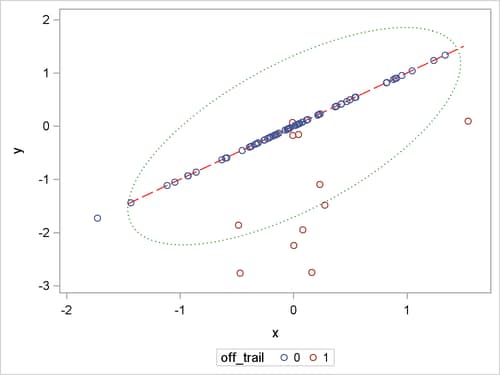
Figure 86.18 exactly identifies the equation that underlies the trail. The analysis projects off-plane points onto the trail and computes their projected robust distances and projected Mahalanobis distances the same way as it does for the in-plane points.
Figure 86.19 shows the relevant distance-distance plot. Robust distance is typically greater than Mahalanobis distance because the sample covariance can be strongly influenced by unusual points that cause the sample covariance to be larger than the MCD covariance.
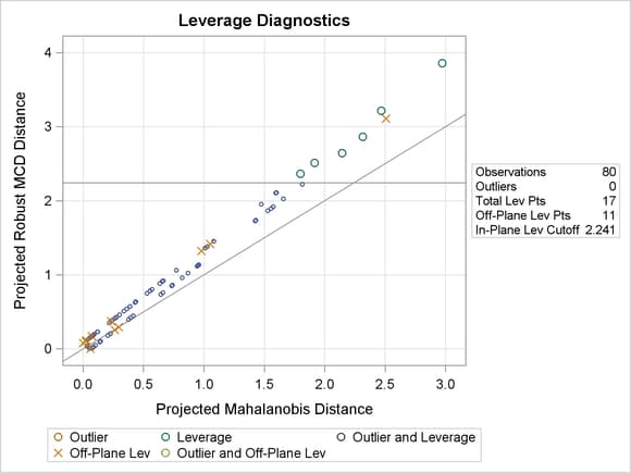
Note: The PROC ROBUSTREG step in this example is used to obtain the leverage diagnostics; the response is not relevant for this analysis.
Through the off-plane and in-plane symbols and the horizontal cutoff line in Figure 86.19, you can separate the children into four groups:
-
on the trail and close to the MCD center
-
on the trail but far away from the MCD center
-
off the trail but close to the MCD center
-
off the trail and far away from the MCD center
The children in the latter three groups are defined as leverage points in PROC ROBUSTREG.
The generalized MCD algorithm follows the same resampling strategy as the canonical MCD algorithm by Rousseeuw and Van Driessen (1999) but with the following modifications:
-
Data are orthonormalized before further processing. The orthonormalized covariates,
 , are defined by
 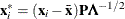 , where
  and
and  are the eigenvector and eigenvalue matrices, respectively, of
  (that is,
  ).
).
-
Let
![\[ S_ h(\bX ^*)={1\over h-1}\sum _{j=1}^ h ({\mb{x}_{i_ j}^*} - {\bar{\mb{x}}^*})’ ({\mb{x}_{i_ j}^*} - {\bar{\mb{x}}^*})= \sum _{j=1}^{p-1}{\lambda _ j \mb{p}_ j{\mb{p}_ j}’} \]](images/statug_rreg0232.png)
denote the covariance and eigendecomposition of a low-dimensional h-subset
 , where
  and the eigenvalues satisfy
![\[ \lambda _1\ge \cdots \ge \lambda _ q>0=\lambda _{q+1}=\cdots =\lambda _ p \]](images/statug_rreg0235.png)
Then, the rank of
 equals q, and the pseudo-determinant of is defined as
  . In finite-precision arithmetic, q is defined as the number of
  ’s where
  is greater than a certain tolerance value. You can specify this tolerance by using the PTOL= suboption of the LEVERAGE option.
-
If
and  are the covariance and center estimates, respectively, then the projected Mahalanobis distance for
  is defined as
![\[ \left[\sum _{j=1}^ q{\left((\mb{x}_ i^* - {\bar{\mb{x}}^*})\mb{p}_ j\right)^2 \over \lambda _ j}\right]^{1/2} \]](images/statug_rreg0242.png)
The generalized algorithm also computes off-plane distance for each
as
![\[ \left[\sum _{j=q+1}^{p}{\left((\mb{x}_ i^* - {\bar{\mb{x}}^*})\mb{p}_ j\right)^2}\right]^{1/2} \]](images/statug_rreg0243.png)
In finite-precision arithmetic,
 in the previous off-plane formula are truncated to zero if they satisfy
![\[ {{\left(({\mb{x}_ i^*} - {\bar{\mb{x}}^*})\mb{p}_ j\right)^2} \over \lambda _ j}\le \mbox{cutoff} \]](images/statug_rreg0245.png)
You can tune this
 by using either the PCUTOFF= or PALPHA= suboption of the LEVERAGE option. The points with zero off-plane distances are called
in-plane points; otherwise, they are called off-plane points. Analogous to ordering all points in terms of their canonical
Mahalanobis distances, for the generalized MCD algorithm the points are first sorted by their off-plane distances, and the
points with the same off-plane distance values are further sorted by their projected Mahalanobis distances.
by using either the PCUTOFF= or PALPHA= suboption of the LEVERAGE option. The points with zero off-plane distances are called
in-plane points; otherwise, they are called off-plane points. Analogous to ordering all points in terms of their canonical
Mahalanobis distances, for the generalized MCD algorithm the points are first sorted by their off-plane distances, and the
points with the same off-plane distance values are further sorted by their projected Mahalanobis distances.
-
Instead of comparing the determinants of h-subset covariance matrices, the generalized algorithm compares both the ranks and pseudo-determinants of the h-subset covariance matrices. If the ranks of two matrices are different, the matrix that has the smaller rank is treated as if its determinant were smaller. If two matrices are of the same rank, they are compared in terms of their pseudo-determinants.
-
Suppose that the
of the minimum determinant is singular. Then the relevant low-dimensional structure or hyperplane can be identified by using
the eigendecomposition of . The eigenvectors that correspond to the nonzero eigenvalues form a basis for the low-dimensional hyperplane. The projected
off-plane distance (POD) for is defined as the off-plane distance that is associated with the  . To provide further leverage analysis on the low-dimensional hyperplane, every is transformed into
  , where
  are the eigenvectors of the . The projected robust distance (PRD) is then computed as the reweighted Mahalanobis distance on all the transformed in-plane
points. The off-plane points are assigned zero weights at the reweighting stage, because they are leverage points by definition.
The in-plane points are classified into two groups, the normal group and the in-plane leverage group. This classification
is made by comparing their projected robust distances with a leverage cutoff value. (For more information, see the section
Leverage-Point and Outlier Detection.) This reweighting process mirrors the one that was proposed by Rousseeuw and Van Driessen (1999). However, the degrees of freedom p for the reweighting critical
are the eigenvectors of the . The projected robust distance (PRD) is then computed as the reweighted Mahalanobis distance on all the transformed in-plane
points. The off-plane points are assigned zero weights at the reweighting stage, because they are leverage points by definition.
The in-plane points are classified into two groups, the normal group and the in-plane leverage group. This classification
is made by comparing their projected robust distances with a leverage cutoff value. (For more information, see the section
Leverage-Point and Outlier Detection.) This reweighting process mirrors the one that was proposed by Rousseeuw and Van Driessen (1999). However, the degrees of freedom p for the reweighting critical  value are replaced by q. You can control the critical value by specifying the MCDCUTOFF= or MCDALPHA= option.
If the data set under investigation has a low-dimensional structure, you can use two ODS objects, DependenceEquations and MCDDependenceEquations, to identify the regressors that are linear combinations of other regressors plus certain constants. The equations in DependenceEquations hold for the entire data set, whereas the equations in MCDDependenceEquations apply only to the majority of the observations.
By using the OPC suboption of the LEVERAGE option, you can request an ODS table called DroppedComponents. Figure 86.20 shows the DroppedComponents table for the Children data set example. This table contains a set of coefficient vectors for regressors, which form a basis of the complementary
space for the relevant low-dimensional structure.
By using the MCDINFO suboption of the LEVERAGE option, you can request that detailed information about the MCD covariance
estimate be displayed in four ODS tables: MCDProfile, MCDCenter, MCDCov, and MCDCorr. Figure 86.21 shows an example of the MCD information tables for the Children data set. The number of dimensions in the table MCDProfile equals the number of nonintercept regressors minus the number
of design-dropped components. The specified value of H is the same as h for the h-subset that you can specify by using the QUANTILE= suboption of the LEVERAGE option in the MODEL statement. The reweighted
H is the number of observations that are actually used to compute the MCD center and MCD covariance after the reweighting
step of the MCD algorithm.