The ROBUSTREG Procedure

MM estimation is a combination of high breakdown value estimation and efficient estimation that was introduced by Yohai (1987). It has the following three steps:
-
Compute an initial (consistent) high breakdown value estimate
 . The ROBUSTREG procedure provides two kinds of estimates as the initial estimate: the LTS estimate and the S estimate. By
default, the LTS estimate is used because of its speed and high breakdown value. The breakdown value of the final MM estimate
is decided by the breakdown value of the initial LTS estimate and the constant
. The ROBUSTREG procedure provides two kinds of estimates as the initial estimate: the LTS estimate and the S estimate. By
default, the LTS estimate is used because of its speed and high breakdown value. The breakdown value of the final MM estimate
is decided by the breakdown value of the initial LTS estimate and the constant  in the
  function. To use the S estimate as the initial estimate, specify the INITEST=S option in the PROC ROBUSTREG statement. In
this case, the breakdown value of the final MM estimate is decided only by the constant . Instead of computing the LTS estimate or the S estimate as the initial estimate, you can also specify the initial estimate
explicitly by using the INEST= option in the PROC ROBUSTREG statement. For more information, see the section INEST= Data Set.
function. To use the S estimate as the initial estimate, specify the INITEST=S option in the PROC ROBUSTREG statement. In
this case, the breakdown value of the final MM estimate is decided only by the constant . Instead of computing the LTS estimate or the S estimate as the initial estimate, you can also specify the initial estimate
explicitly by using the INEST= option in the PROC ROBUSTREG statement. For more information, see the section INEST= Data Set.
-
Find
 such that
![\[ {1\over n-p} \sum _{i=1}^ n \chi \left( {y_ i - \mb{x}_ i’ {\hat\btheta }’ \over {\hat\sigma }’ }\right) = \beta \]](images/statug_rreg0186.png)
where
 .
.
The ROBUSTREG procedure provides two choices for
: Tukey’s bisquare function and Yohai’s optimal function.
Tukey’s bisquare function, which you can specify by using the option CHIF=TUKEY, is
![\[ \chi _{k_0}(s) = \left\{ \begin{array}{ll} 3({s\over k_0})^2 - 3({s\over k_0})^4 + ({s\over k_0})^6& {\mbox{if }} |s| \leq k_0 \\ 1 & {\mbox{ otherwise }} \end{array} \right. \]](images/statug_rreg0188.png)
where
can be specified by using the K0= option. The default  is 2.9366, such that the asymptotically consistent scale estimate has a breakdown value of 25%.
Yohai’s optimal function, which you can specify by using the option CHIF=YOHAI, is
![\[ \chi _{k_0}(s) = \left\{ \begin{array}{lll} {s^2 \over 2} & {\mbox{if }} |s| \leq 2 k_0 \\ k_0^2 [ b_0 + b_1({s\over k_0})^2 + b_2({s\over k_0})^4 & \\ + b_3({s\over k_0})^6 + b_4({s\over k_0})^8] & {\mbox{if }} 2 k_0 < |s| \leq 3 k_0\\ 3.25 k_0^2 & {\mbox{if }} |s| >3 k_0 \end{array} \right. \]](images/statug_rreg0147.png)
where
 ,
,  ,
,  ,
,  , and
, and  . You can use the K0= option to specify . The default is 0.7405, such that the asymptotically consistent scale estimate has a breakdown value of 25%.
-
Find a local minimum
 of
of
![\[ Q_{\mathit{MM}} = \sum _{i=1}^ n \rho \left( {y_ i - \mb{x}_ i’ \btheta \over {\hat\sigma }’} \right) \]](images/statug_rreg0190.png)
such that
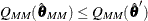 . The algorithm for M estimation is used here.
The ROBUSTREG procedure provides two choices for
 : Tukey’s bisquare function and Yohai’s optimal function.
Tukey’s bisquare function, which you can specify by using the option CHIF=TUKEY, is
![\[ \rho (s) = \chi _{k_1}(s) = \left\{ \begin{array}{ll} 3({s\over k_1})^2 - 3({s\over k_1})^4 + ({s\over k_1})^6 & {\mbox{if }} |s| \leq k_1 \\ 1 & {\mbox{ otherwise }} \end{array} \right. \]](images/statug_rreg0192.png)
where
 can be specified by using the K1= option. The default is 3.440 such that the MM estimate has 85% asymptotic efficiency with the Gaussian distribution.
Yohai’s optimal function, which you can specify by using the option CHIF=YOHAI, is
![\[ \rho (s) = \chi _{k_1}(s) = \left\{ \begin{array}{lll} {s^2 \over 2} & {\mbox{if }} |s| \leq 2 k_1 \\ k_1^2 [ b_0 + b_1({s\over k_1})^2 + b_2({s\over k_1})^4 & \\ + b_3({s\over k_1})^6 + b_4({s\over k_1})^8] & {\mbox{if }} 2 k_1 < |s| \leq 3 k_1\\ 3.25 k_1^2 & {\mbox{if }} |s| >3 k_1 \end{array} \right. \]](images/statug_rreg0194.png)
where
can be specified by using the K1= option. The default is 0.868 such that the MM estimate has 85% asymptotic efficiency with the Gaussian distribution.
The initial LTS estimate is computed using the algorithm described in the section LTS Estimate. You can control the quantile of the LTS estimate by specifying the option INITH=h, where h is an integer between ![]() and
and ![]() . By default,
. By default, ![]() , which corresponds to a breakdown value of around 25%.
, which corresponds to a breakdown value of around 25%.
The initial S estimate is computed using the algorithm described in the section S Estimate. You can control the breakdown value and efficiency of this initial S estimate by the constant ![]() , which you can specify by using the K0= option.
, which you can specify by using the K0= option.
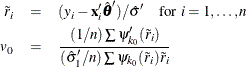
The scale parameter ![]() is solved by an iterative algorithm
is solved by an iterative algorithm
where ![]() .
.
After the scale parameter is computed, the iteratively reweighted least squares (IRLS) algorithm with fixed scale parameter is used to compute the final MM estimate.
In the iterative algorithm for the scale parameter, the relative change of the scale parameter controls the convergence.
In the iteratively reweighted least squares algorithm, the same convergence criteria for the M estimate that are used before are used here.
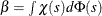
Although the final MM estimate inherits the high breakdown value property, its bias from the distortion of the outliers can
be high. Yohai, Stahel, and Zamar (1991) introduced a bias test. The ROBUSTREG procedure implements this test when you specify the BIASTEST= option in the PROC ROBUSTREG
statement. This test is based on the initial scale estimate ![]() and the final scale estimate
and the final scale estimate ![]() , which is the solution of
, which is the solution of
Let ![]() and
and ![]() . Compute
. Compute
Let
Standard asymptotic theory shows that T approximately follows a ![]() distribution with p degrees of freedom. If T exceeds the
distribution with p degrees of freedom. If T exceeds the ![]() quantile
quantile ![]() of the
of the ![]() distribution with p degrees of freedom, then the ROBUSTREG procedure gives a warning and recommends that you use other methods. Otherwise, the
final MM estimate and the initial scale estimate are reported. You can specify
distribution with p degrees of freedom, then the ROBUSTREG procedure gives a warning and recommends that you use other methods. Otherwise, the
final MM estimate and the initial scale estimate are reported. You can specify ![]() by using the ALPHA= option after the BIASTEST= option. By default, ALPHA=0.99.
by using the ALPHA= option after the BIASTEST= option. By default, ALPHA=0.99.
Because the MM estimate is computed as an M estimate with a known scale in the last step, the asymptotic covariance for the M estimate can be used here for the asymptotic covariance of the MM estimate. Besides the three estimators H1, H2, and H3 as described in the section Asymptotic Covariance and Confidence Intervals, a weighted covariance estimator H4 is available. H4 is calculated as
where ![]() is the correction factor and
is the correction factor and ![]() ,
, ![]() .
.
You can specify these estimators by using the option ASYMPCOV=[H1 | H2 | H3 | H4]. The ROBUSTREG procedure uses H4 as the default. Confidence intervals for estimated parameters are computed from the diagonal elements of the estimated asymptotic covariance matrix.
The robust version of R square for the MM estimate is defined as
![\[ R^2 = {{\sum \rho \left({y_ i-{\hat\mu } \over {\hat s}}\right) - \sum \rho \left({y_ i-\mb{x}_ i’ {\hat\btheta } \over {\hat s}}\right) \over \sum \rho \left({y_ i-{\hat\mu } \over {\hat s}}\right)}} \]](images/statug_rreg0080.png)
and the robust deviance is defined as the optimal value of the objective function on the ![]() scale,
scale,
where ![]() ,
, ![]() is the MM estimator of
is the MM estimator of ![]() ,
, ![]() is the MM estimator of location, and
is the MM estimator of location, and ![]() is the MM estimator of the scale parameter in the full model.
is the MM estimator of the scale parameter in the full model.
For MM estimation, you can use the same ![]() test and
test and ![]() test that used for M estimation. For more information, see the section Linear Tests.
test that used for M estimation. For more information, see the section Linear Tests.
For MM estimation, you can use the same two model selection methods that are used for M estimation. For more information, see the section Model Selection.