The REG Procedure
- Overview
-
Getting Started

-
Syntax
-
DetailsMissing ValuesInput Data SetsOutput Data SetsInteractive AnalysisModel-Selection MethodsCriteria Used in Model-Selection MethodsLimitations in Model-Selection MethodsParameter Estimates and Associated StatisticsPredicted and Residual ValuesModels of Less Than Full RankCollinearity DiagnosticsModel Fit and Diagnostic StatisticsInfluence StatisticsReweighting Observations in an AnalysisTesting for HeteroscedasticityTesting for Lack of FitMultivariate TestsAutocorrelation in Time Series DataComputations for Ridge Regression and IPC AnalysisConstruction of Q-Q and P-P PlotsComputational MethodsComputer Resources in Regression AnalysisDisplayed OutputPlot Options Superseded by ODS GraphicsODS Table NamesODS Graphics
-
Examples
- References
The display of the predicted values and residuals is controlled by the P, R, CLM, and CLI options in the MODEL statement. The P option causes PROC REG to display the observation number, the ID value (if an ID statement is used), the actual value, the predicted value, and the residual. The R, CLI, and CLM options also produce the items under the P option. Thus, P is unnecessary if you use one of the other options.
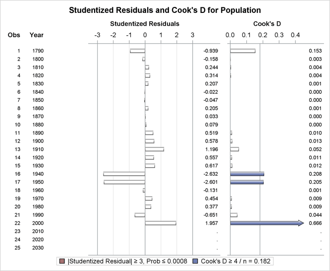
The R option requests more detail, especially about the residuals. The standard errors of the mean predicted value and the residual are displayed. The studentized residual, which is the residual divided by its standard error, is both displayed and plotted. A measure of influence, Cook’s D, is displayed and plotted. Cook’s D measures the change to the estimates that results from deleting each observation (Cook, 1977, 1979). This statistic is very similar to DFFITS.
The CLM option requests that PROC REG display the ![]() % lower and upper confidence limits for the mean predicted values. This accounts for the variation due to estimating the parameters
only. If you want a
% lower and upper confidence limits for the mean predicted values. This accounts for the variation due to estimating the parameters
only. If you want a ![]() % confidence interval for observed values, then you can use the CLI option, which adds in the variability of the error term.
The
% confidence interval for observed values, then you can use the CLI option, which adds in the variability of the error term.
The ![]() level can be specified with the ALPHA= option in the PROC REG
or MODEL
statement.
level can be specified with the ALPHA= option in the PROC REG
or MODEL
statement.
You can use these statistics in PLOT and PAINT statements. This is useful in performing a variety of regression diagnostics. For definitions of the statistics produced by these options, see Chapter 4: Introduction to Regression Procedures.
The following statements use the U.S. population data found in the section Polynomial Regression. The results are shown in Figure 85.33 and Figure 85.34.
ods graphics on;

data USPop2;
   input Year @@;
   YearSq=Year*Year;
   datalines;
2010 2020 2030
;

data USPop2;
   set USPopulation USPop2;
run;

proc reg data=USPop2;
   id Year;
   model Population=Year YearSq / r cli clm;
run;
Figure 85.33: Regression Using the R, CLI, and CLM Options
| Analysis of Variance | |||||
|---|---|---|---|---|---|
| Source | DF | Sum of Squares |
Mean Square |
F Value | Pr > F |
| Model | 2 | 159529 | 79765 | 8864.19 | <.0001 |
| Error | 19 | 170.97193 | 8.99852 | ||
| Corrected Total | 21 | 159700 | |||
| Root MSE | 2.99975 | R-Square | 0.9989 |
|---|---|---|---|
| Dependent Mean | 94.64800 | Adj R-Sq | 0.9988 |
| Coeff Var | 3.16938 |
| Parameter Estimates | |||||
|---|---|---|---|---|---|
| Variable | DF | Parameter Estimate |
Standard Error |
t Value | Pr > |t| |
| Intercept | 1 | 21631 | 639.50181 | 33.82 | <.0001 |
| Year | 1 | -24.04581 | 0.67547 | -35.60 | <.0001 |
| YearSq | 1 | 0.00668 | 0.00017820 | 37.51 | <.0001 |
Figure 85.34: Regression Using the R, CLI, and CLM Options
| Output Statistics | ||||||||||||
|---|---|---|---|---|---|---|---|---|---|---|---|---|
| Obs | Year | Dependent Variable |
Predicted Value |
Std Error Mean Predict |
95% CL Mean | 95% CL Predict | Residual | Std Error Residual |
Student Residual |
Cook's D | ||
| 1 | 1790 | 3.93 | 6.2127 | 1.7565 | 2.5362 | 9.8892 | -1.0631 | 13.4884 | -2.2837 | 2.432 | -0.939 | 0.153 |
| 2 | 1800 | 5.31 | 5.7226 | 1.4560 | 2.6751 | 8.7701 | -1.2565 | 12.7017 | -0.4146 | 2.623 | -0.158 | 0.003 |
| 3 | 1810 | 7.24 | 6.5694 | 1.2118 | 4.0331 | 9.1057 | -0.2021 | 13.3409 | 0.6696 | 2.744 | 0.244 | 0.004 |
| 4 | 1820 | 9.64 | 8.7531 | 1.0305 | 6.5963 | 10.9100 | 2.1144 | 15.3918 | 0.8849 | 2.817 | 0.314 | 0.004 |
| 5 | 1830 | 12.87 | 12.2737 | 0.9163 | 10.3558 | 14.1916 | 5.7087 | 18.8386 | 0.5923 | 2.856 | 0.207 | 0.001 |
| 6 | 1840 | 17.07 | 17.1311 | 0.8650 | 15.3207 | 18.9415 | 10.5968 | 23.6655 | -0.0621 | 2.872 | -0.022 | 0.000 |
| 7 | 1850 | 23.19 | 23.3254 | 0.8613 | 21.5227 | 25.1281 | 16.7932 | 29.8576 | -0.1344 | 2.873 | -0.047 | 0.000 |
| 8 | 1860 | 31.44 | 30.8566 | 0.8846 | 29.0051 | 32.7080 | 24.3107 | 37.4024 | 0.5864 | 2.866 | 0.205 | 0.001 |
| 9 | 1870 | 39.82 | 39.7246 | 0.9163 | 37.8067 | 41.6425 | 33.1597 | 46.2896 | 0.0934 | 2.856 | 0.033 | 0.000 |
| 10 | 1880 | 50.16 | 49.9295 | 0.9436 | 47.9545 | 51.9046 | 43.3476 | 56.5114 | 0.2255 | 2.847 | 0.079 | 0.000 |
| 11 | 1890 | 62.95 | 61.4713 | 0.9590 | 59.4641 | 63.4785 | 54.8797 | 68.0629 | 1.4757 | 2.842 | 0.519 | 0.010 |
| 12 | 1900 | 75.99 | 74.3499 | 0.9590 | 72.3427 | 76.3571 | 67.7583 | 80.9415 | 1.6441 | 2.842 | 0.578 | 0.013 |
| 13 | 1910 | 91.97 | 88.5655 | 0.9436 | 86.5904 | 90.5405 | 81.9836 | 95.1473 | 3.4065 | 2.847 | 1.196 | 0.052 |
| 14 | 1920 | 105.71 | 104.1178 | 0.9163 | 102.2000 | 106.0357 | 97.5529 | 110.6828 | 1.5922 | 2.856 | 0.557 | 0.011 |
| 15 | 1930 | 122.78 | 121.0071 | 0.8846 | 119.1556 | 122.8585 | 114.4612 | 127.5529 | 1.7679 | 2.866 | 0.617 | 0.012 |
| 16 | 1940 | 131.67 | 139.2332 | 0.8613 | 137.4305 | 141.0359 | 132.7010 | 145.7654 | -7.5642 | 2.873 | -2.632 | 0.208 |
| 17 | 1950 | 151.33 | 158.7962 | 0.8650 | 156.9858 | 160.6066 | 152.2618 | 165.3306 | -7.4712 | 2.872 | -2.601 | 0.205 |
| 18 | 1960 | 179.32 | 179.6961 | 0.9163 | 177.7782 | 181.6139 | 173.1311 | 186.2610 | -0.3731 | 2.856 | -0.131 | 0.001 |
| 19 | 1970 | 203.21 | 201.9328 | 1.0305 | 199.7759 | 204.0896 | 195.2941 | 208.5715 | 1.2782 | 2.817 | 0.454 | 0.009 |
| 20 | 1980 | 226.54 | 225.5064 | 1.2118 | 222.9701 | 228.0427 | 218.7349 | 232.2779 | 1.0356 | 2.744 | 0.377 | 0.009 |
| 21 | 1990 | 248.71 | 250.4168 | 1.4560 | 247.3693 | 253.4644 | 243.4378 | 257.3959 | -1.7068 | 2.623 | -0.651 | 0.044 |
| 22 | 2000 | 281.42 | 276.6642 | 1.7565 | 272.9877 | 280.3407 | 269.3884 | 283.9400 | 4.7578 | 2.432 | 1.957 | 0.666 |
| 23 | 2010 | . | 304.2484 | 2.1073 | 299.8377 | 308.6591 | 296.5754 | 311.9214 | . | . | . | . |
| 24 | 2020 | . | 333.1695 | 2.5040 | 327.9285 | 338.4104 | 324.9910 | 341.3479 | . | . | . | . |
| 25 | 2030 | . | 363.4274 | 2.9435 | 357.2665 | 369.5883 | 354.6310 | 372.2238 | . | . | . | . |
After producing the usual analysis of variance and parameter estimates tables (Figure 85.33), the procedure displays the results of requesting the options for predicted and residual values (Figure 85.34). For each observation, the requested information is shown. Note that the ID variable is used to identify each observation. Also note that, for observations with missing dependent variables, the predicted value, standard error of the predicted value, and confidence intervals for the predicted value are still available.
The studentized residuals and Cook’s D statistics in Figure 85.34 and Figure 85.35 are displayed as a result of specifying the R option. The large absolute studentized residuals for 1940 and 1950 (best seen in Figure 85.35) indicate that the overall model is inadequate for explaining the population in these two years. You can use ODS Graphics to obtain plots of studentized residuals by predicted values or leverage; see Example 85.1 for a similar example.