The QUANTREG Procedure

The QUANTREG procedure uses quantile regression to model the effects of covariates on the conditional quantiles of a response variable.
Quantile regression was introduced by Koenker and Bassett (1978) as an extension of ordinary least squares (OLS) regression, which models the relationship between one or more covariates
X and the conditional mean of the response variable Y given ![]() . Quantile regression extends the OLS regression to model the conditional quantiles of the response variable, such as the median or the 90th percentile. Quantile regression is particularly useful when the
rate of change in the conditional quantile, expressed by the regression coefficients, depends on the quantile.
. Quantile regression extends the OLS regression to model the conditional quantiles of the response variable, such as the median or the 90th percentile. Quantile regression is particularly useful when the
rate of change in the conditional quantile, expressed by the regression coefficients, depends on the quantile.
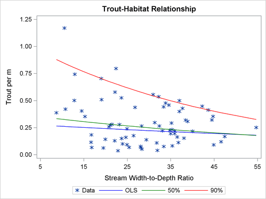
Figure 83.1 illustrates an ecological study in which modeling upper conditional quantiles reveals additional information. The points represent measurements of trout density and stream width-to-depth ratio that were taken at 13 streams over seven years.
As analyzed by Dunham, Cade, and Terrell (2002), both the ratio and the trout density depend on a number of unmeasured limiting factors that are related to the integrity of stream habitat. The interaction of these factors results in unequal variances for the conditional distributions of density given the ratio. When the ratio is the "active" limiting effect, changes in the upper conditional percentiles of density provide a better estimate of this effect than changes in the conditional mean.
The red and green curves represent the conditional 90th and 50th percentiles of density as determined by the QUANTREG procedure. The analysis was done by using a simple linear regression model for the logarithm of density. (The curves in Figure 83.1 were obtained by transforming the fitted lines back to the original scale. For more information, see the section Analysis of Fish-Habitat Relationships.) The slope parameter for the 90th percentile has an estimated value of –0.0215 and is significant with a p-value less than 0.01. On the other hand, the slope parameter for the 50th percentile is not significantly different from 0. Similarly, the slope parameter for the mean, which is obtained with OLS regression, is not significantly different from 0.
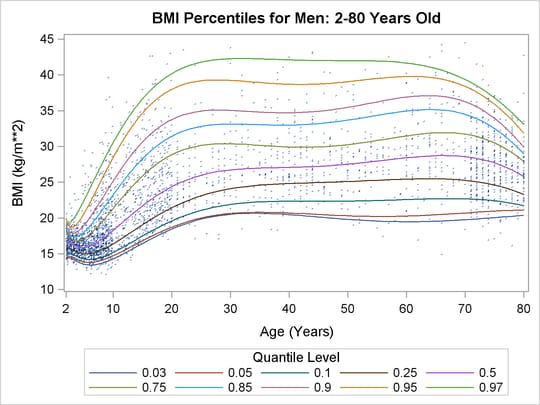
Quantile regression is especially useful when the data are heterogeneous in the sense that the tails and the central location of the conditional distributions vary differently with the covariates. An even more pronounced example of heterogeneity is shown in Figure 83.2, which plots the body mass index of 8,250 men versus their age.
Here, both upper (overweight) and lower (underweight) conditional quantiles are important because they provide the basis for developing growth charts and establishing health standards. The curves in Figure 83.2 were determined by using the QUANTREG procedure to perform polynomial quantile regression. For more information, see the section Growth Charts for Body Mass Index. Clearly, the rate of change with age (as expressed by the regression coefficients), particularly for ages less than 20, is different for each conditional quantile.
Heterogeneous data occur in many fields, including biomedicine, econometrics, survival analysis, and ecology. Quantile regression, which includes median regression as a special case, provides a complete picture of the covariate effect when a set of percentiles is modeled. So it can capture important features of the data that might be missed by models that average over the conditional distribution.
Because it makes no distributional assumption about the error term in the model, quantile regression offers considerable model robustness. The assumption of normality, which is often made with OLS regression in order to compute conditional quantiles as offsets from the mean, forces a common set of regression coefficients for all the quantiles. Obviously, quantiles with common slopes would be inappropriate in the preceding examples.
Quantile regression is also flexible because it does not involve a link function that relates the variance and the mean of the response variable. Generalized linear models, which you can fit with the GENMOD procedure, require both a link function and a distributional assumption such as the normal or Poisson distribution. The goal of generalized linear models is inference about the regression parameters in the linear predictor for the mean of the population. In contrast, the goal of quantile regression is inference about regression coefficients for the conditional quantiles of a response variable that is usually assumed to be continuous.
Quantile regression also offers a degree of data robustness. Unlike OLS regression, quantile regression is robust to extreme points in the response direction (outliers). However, it is not robust to extreme points in the covariate space (leverage points). When both types of robustness are of concern, consider using the ROBUSTREG procedure (Chapter 86: The ROBUSTREG Procedure.)
Unlike OLS regression, quantile regression is equivariant to monotone transformations of the response variable. For example, as illustrated in the trout example, the logarithm of the 90th conditional percentile of trout density is the 90th conditional percentile of the logarithm of density.
Quantile regression cannot be carried out simply by segmenting the unconditional distribution of the response variable and then obtaining least squares fits for the subsets. This approach leads to disastrous results when, for example, the data include outliers. In contrast, quantile regression uses all of the data for fitting quantiles, even the extreme quantiles.