The QUANTREG Procedure

Consider the linear model
where ![]() and
and ![]() are p- and q-dimensional unknown parameters and
are p- and q-dimensional unknown parameters and ![]() ,
, ![]() , are errors with unknown density function
, are errors with unknown density function ![]() . Let
. Let ![]() , and let
, and let ![]() and
and ![]() be the parameter estimates for
be the parameter estimates for ![]() and
and ![]() , respectively at the
, respectively at the ![]() quantile. The covariance matrix
quantile. The covariance matrix ![]() for the parameter estimates is partitioned correspondingly as
for the parameter estimates is partitioned correspondingly as ![]() with
with ![]() ; and
; and ![]()
Three tests are available in the QUANTREG procedure for the linear null hypothesis ![]() at the
at the ![]() quantile:
quantile:
-
The Wald test statistic, which is based on the estimated coefficients for the unrestricted model, is given by
![\[ T_ W(\tau ) = {\hat\bbeta _2^{\prime }(\tau )} {\hat\bSigma (\tau )}^{-1} {\hat\bbeta _2(\tau )} \]](images/statug_qreg0278.png)
where
 is an estimator of the covariance of
  . The QUANTREG procedure provides two estimators for the covariance, as described in the previous section. The estimator that
is based on the asymptotic covariance is
. The QUANTREG procedure provides two estimators for the covariance, as described in the previous section. The estimator that
is based on the asymptotic covariance is
![\[ {\hat\bSigma (\tau )} = {\frac1n} {\hat\omega (\tau )}^{2} {\bOmega }^{22} \]](images/statug_qreg0281.png)
where
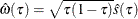 and
and  is the estimated sparsity function. The estimator that is based on the bootstrap covariance is the empirical covariance of
the MCMB samples.
is the estimated sparsity function. The estimator that is based on the bootstrap covariance is the empirical covariance of
the MCMB samples.
-
The likelihood ratio test is based on the difference between the objective function values in the restricted and unrestricted models. Let
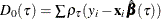 , and let
 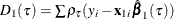 . Set
. Set
![\[ T_{\mr{LR}}(\tau ) = 2 ({\tau (1-\tau )}{\hat s(\tau )})^{-1} ( D_1(\tau ) - D_0(\tau ) ) \]](images/statug_qreg0286.png)
where
is the estimated sparsity function.
-
The rank test statistic is given by
![\[ T_ R(\tau ) = \bS _ n^{\prime } \bM _ n^{-1} \bS _ n/A^2(\varphi ) \]](images/statug_qreg0287.png)
where
![\[ \bS _ n=n^{-1/2} (\bX _2 - \hat{\bX }_2)^{\prime } \hat{\mb{b}}_ n \]](images/statug_qreg0288.png)
![\[ \bPsi =\mr{diag}(f_ i(Q_{y_ i}(\tau |\mb{x}_{1i},\mb{x}_{2i}))) \]](images/statug_qreg0289.png)
![\[ \hat{\bX }_2 = \bX _1(\bX _1^{\prime } \bPsi {\bX _1})^{-1}\bX _1^{\prime } {\bX _2} \]](images/statug_qreg0290.png)
![\[ \bM _ n = (\bX _2 - \hat{\bX }_2) (\bX _2 - \hat{\bX }_2)^{\prime }/n \]](images/statug_qreg0291.png)
![\[ \hat{\mb{b}}_{ni} = \int _0^1 \hat{\mb{a}}_{ni}(t) d \varphi (t) \]](images/statug_qreg0292.png)
![\[ \hat{\mb{a}}(t) = \max _ a \{ \mb{y}^{\prime }\mb{a} | \bX _1^{\prime }\mb{a} = (1-t)\bX _1^{\prime }\mb{e}, \ \mb{a}\in [0,1]^ n \} \]](images/statug_qreg0293.png)
![\[ A^2(\varphi ) = \int _0^1 (\varphi (t) - \bar{\varphi }(t))^2 dt \]](images/statug_qreg0294.png)
![\[ \bar{\varphi }(t) = \int _0^1 \varphi (t) dt \]](images/statug_qreg0295.png)
and
 is one of the following score functions:
-
Wilcoxon scores:

-
normal scores:
 , where
  is the normal distribution function
-
sign scores:
-
tau scores:
 .
.
The rank test statistic
 , unlike Wald tests or likelihood ratio tests, requires no estimation of the nuisance parameter
  under iid error models (Gutenbrunner et al., 1993).
-
Koenker and Machado (1999) prove that the three test statistics (![]() , and
, and ![]() ) are asymptotically equivalent and that their distributions converge to
) are asymptotically equivalent and that their distributions converge to ![]() under the null hypothesis, where q is the dimension of
under the null hypothesis, where q is the dimension of ![]() .
.
After you obtain the parameter estimates for several quantiles specified in the MODEL statement, you can test whether there
are significant differences for the estimates for the same covariates across the quantiles. For example, if you want to test
whether the parameters ![]() are the same across quantiles, the null hypothesis
are the same across quantiles, the null hypothesis ![]() can be written as
can be written as ![]() , where
, where ![]() are the quantiles specified in the MODEL statement. See Koenker and Bassett (1982a) for details.
are the quantiles specified in the MODEL statement. See Koenker and Bassett (1982a) for details.