Using the Output Delivery System
-
Overview

-
ExamplesCreating HTML Output with ODSSelecting ODS Tables for DisplayExcluding ODS Tables from DisplayCreating an Output Data Set from an ODS TableCreating an Output Data Set: Subsetting the DataRUN-Group ProcessingODS Output Data Sets and Using PROC TEMPLATE to Customize OutputHTML Output with Hyperlinks between TablesHTML Output with Graphics and HyperlinksCorrelation and Covariance Matrices
- References
You can use ODS statements, the DATA step, and PROC TEMPLATE to modify the appearance of your displayed tables or to display results in forms that are not directly produced by any procedure. The following example, similar to that given in Olinger and Tobias (1998), runs an analysis with PROC GLM. This example has several parts. It creates output data sets with the ODS OUTPUT statement, combines and manipulates those data sets, displays the results by using a standard SAS template, modifies a template by using PROC TEMPLATE, and displays the output data sets by using the modified template. Each step works toward the final goal of taking multiple tables and creating a custom display of those tables in a way that cannot be done directly by PROC GLM.
The following statements create a SAS data set named Histamine that contains the experimental data:
title1 'Histamine Study';

data Histamine;
   input Drug $12. Depleted $ hist0 hist1 hist3 hist5;
   logHist0 = log(hist0); logHist1 = log(Hist1);
   logHist3 = log(hist3); logHist5 = log(Hist5);
   datalines;
Morphine      N  .04  .20  .10  .08
Morphine      N  .02  .06  .02  .02
Morphine      N  .07 1.40  .48  .24
Morphine      N  .17  .57  .35  .24
Morphine      Y  .10  .09  .13  .14
Morphine      Y  .07  .07  .06  .07
Morphine      Y  .05  .07  .06  .07
Trimethaphan  N  .03  .62  .31  .22
Trimethaphan  N  .03 1.05  .73  .60
Trimethaphan  N  .07  .83 1.07  .80
Trimethaphan  N  .09 3.13 2.06 1.23
Trimethaphan  Y  .10  .09  .09  .08
Trimethaphan  Y  .08  .09  .09  .10
Trimethaphan  Y  .13  .10  .12  .12
Trimethaphan  Y  .06  .05  .05  .05
;
The data set comes from a preclinical drug experiment (Cole and Grizzle, 1966). In order to study the effect of two different drugs on histamine levels in the blood, researchers administer the drugs to 13 animals and measure the levels of histamine in the animals’ blood after 0, 1, 3, and 5 minutes. The response variable is the logarithm of the histamine level.
In the analysis that follows, PROC GLM is used to perform a repeated measures analysis, naming the drug and depletion status as between-subject factors in the MODEL statement and naming post-administration measurement time as the within-subject factor. For more information about this study and its analysis, see Example 45.7 in Chapter 45: The GLM Procedure.
The following PROC GLM statements begin the analysis:
ods graphics off;
ods trace output;

proc glm data=Histamine;
   class Drug Depleted;
   model LogHist0--LogHist5 = Drug Depleted Drug*Depleted / nouni;
   repeated Time 4 (0 1 3 5) polynomial / summary printe;
run; quit;
The portion of the trace output that contains the fully qualified name paths is shown next:
   Path:       GLM.Data.ClassLevels
   Path:       GLM.Data.NObs
   Path:       GLM.Repeated.RepeatedLevelInfo
   Path:       GLM.Repeated.PartialCorr
   Path:       GLM.Repeated.MANOVA.Model.Error.ErrorSSCP
   Path:       GLM.Repeated.MANOVA.Model.Error.PartialCorr
   Path:       GLM.Repeated.MANOVA.Model.Error.Sphericity
   Path:       GLM.Repeated.MANOVA.Model.Time.MultStat
   Path:       GLM.Repeated.MANOVA.Model.Time_Drug.MultStat
   Path:       GLM.Repeated.MANOVA.Model.Time_Depleted.MultStat
   Path:       GLM.Repeated.MANOVA.Model.Time_Drug_Depleted.MultStat
   Path:       GLM.Repeated.BetweenSubjects.ModelANOVA
   Path:       GLM.Repeated.WithinSubject.ModelANOVA
   Path:       GLM.Repeated.WithinSubject.Epsilons
   Path:       GLM.Repeated.Summary.Time_1.ModelANOVA
   Path:       GLM.Repeated.Summary.Time_2.ModelANOVA
   Path:       GLM.Repeated.Summary.Time_3.ModelANOVA
The goal here is to output the within-subjects multivariate statistics and the between-subjects ANOVA table to SAS data sets for use in subsequent steps. The following statements run the analysis and save the desired results to output data sets:
ods select none;

proc glm data=Histamine;
   class Drug Depleted;
   model LogHist0--LogHist5 = Drug Depleted Drug*Depleted / nouni;
   repeated Time 4 (0 1 3 5) polynomial / summary printe;
   ods output MultStat                   = HistWithin
              BetweenSubjects.ModelANOVA = HistBetween;
run; quit;

ods select all;
No output is displayed due to the ODS SELECT statements. The ODS OUTPUT statement creates two SAS data sets, named HistWithin and HistBetween, from the two ODS tables. This analysis creates the following tables:
   Path:       GLM.Repeated.MANOVA.Model.Time.MultStat
   Path:       GLM.Repeated.MANOVA.Model.Time_Drug.MultStat
   Path:       GLM.Repeated.MANOVA.Model.Time_Depleted.MultStat
   Path:       GLM.Repeated.MANOVA.Model.Time_Drug_Depleted.MultStat
   Path:       GLM.Repeated.BetweenSubjects.ModelANOVA
Here is the full trace output for the model ANOVA table:
   Output Added:
   -------------
   Name:       ModelANOVA
   Label:      Type III Model ANOVA
   Template:   stat.GLM.Tests
   Path:       GLM.Repeated.BetweenSubjects.ModelANOVA
   -------------
All of the multivariate test results are routed to the HistWithin data set because all multivariate test tables are named MultStat, even though they occur in different directories in the
output directory hierarchy. Only the between-subject ANOVA table appears in the HistBetween data set, even though there are also other tables named ModelANOVA. ODS selects just the one specific table for the HistBetween data set because of the partial name path (BetweenSubjects.ModelANOVA) in the second specification. For more information about names and qualified path names, see the discussion in the section
The ODS Statement.
The following statements show the names and the variable labels for the two data sets and produce Output 20.7.1:
proc contents data=HistBetween varnum;
   ods select position;
run;

proc contents data=HistWithin varnum;
   ods select position;
run;
Output 20.7.1: Variable Names and Labels for the Two Data Sets
| Histamine Study |
| Variables in Creation Order | |||||
|---|---|---|---|---|---|
| # | Variable | Type | Len | Format | Label |
| 1 | Hypothesis | Char | 32 | ||
| 2 | Error | Char | 55 | ||
| 3 | Statistic | Char | 22 | ||
| 4 | Value | Num | 8 | 12.8 | |
| 5 | FValue | Num | 8 | 7.2 | F Value |
| 6 | NumDF | Num | 8 | BEST6. | Num DF |
| 7 | DenDF | Num | 8 | BEST6. | Den DF |
| 8 | ProbF | Num | 8 | PVALUE6.4 | Pr > F |
| 9 | PValue | Num | 8 | PVALUE6.4 | P-Value |
The following statements create a new data set that contains the two data sets created in the preceding PROC GLM step and display the results in Output 20.7.2:
title2 'The Combined Data Set';

data temp1;
   set HistBetween HistWithin;
run;

proc print label;
run;
Output 20.7.2: Listing of the Combined Data Set: Histamine Study
| Histamine Study |
| The Combined Data Set |
| Obs | Dependent | HypothesisType | Source | DF |
|---|---|---|---|---|
| 1 | BetweenSubjects | 3 | Drug | 1 |
| 2 | BetweenSubjects | 3 | Depleted | 1 |
| 3 | BetweenSubjects | 3 | Drug*Depleted | 1 |
| 4 | BetweenSubjects | 3 | Error | 11 |
| 5 | . | . | ||
| 6 | . | . | ||
| 7 | . | . | ||
| 8 | . | . | ||
| 9 | . | . | ||
| 10 | . | . | ||
| 11 | . | . | ||
| 12 | . | . | ||
| 13 | . | . | ||
| 14 | . | . | ||
| 15 | . | . | ||
| 16 | . | . | ||
| 17 | . | . | ||
| 18 | . | . | ||
| 19 | . | . | ||
| 20 | . | . |
| Histamine Study |
| The Combined Data Set |
| Obs | Type III SS | Mean Square | F Value | Pr > F | Hypothesis | Error |
|---|---|---|---|---|---|---|
| 1 | 5.99336243 | 5.99336243 | 2.71 | 0.1281 | ||
| 2 | 15.44840703 | 15.44840703 | 6.98 | 0.0229 | ||
| 3 | 4.69087508 | 4.69087508 | 2.12 | 0.1734 | ||
| 4 | 24.34683348 | 2.21334850 | _ | _ | ||
| 5 | . | . | 24.03 | 0.0001 | Time | Error SSCP Matrix |
| 6 | . | . | 24.03 | 0.0001 | Time | Error SSCP Matrix |
| 7 | . | . | 24.03 | 0.0001 | Time | Error SSCP Matrix |
| 8 | . | . | 24.03 | 0.0001 | Time | Error SSCP Matrix |
| 9 | . | . | 5.78 | 0.0175 | Time_Drug | Error SSCP Matrix |
| 10 | . | . | 5.78 | 0.0175 | Time_Drug | Error SSCP Matrix |
| 11 | . | . | 5.78 | 0.0175 | Time_Drug | Error SSCP Matrix |
| 12 | . | . | 5.78 | 0.0175 | Time_Drug | Error SSCP Matrix |
| 13 | . | . | 21.31 | 0.0002 | Time_Depleted | Error SSCP Matrix |
| 14 | . | . | 21.31 | 0.0002 | Time_Depleted | Error SSCP Matrix |
| 15 | . | . | 21.31 | 0.0002 | Time_Depleted | Error SSCP Matrix |
| 16 | . | . | 21.31 | 0.0002 | Time_Depleted | Error SSCP Matrix |
| 17 | . | . | 12.48 | 0.0015 | Time_Drug_Depleted | Error SSCP Matrix |
| 18 | . | . | 12.48 | 0.0015 | Time_Drug_Depleted | Error SSCP Matrix |
| 19 | . | . | 12.48 | 0.0015 | Time_Drug_Depleted | Error SSCP Matrix |
| 20 | . | . | 12.48 | 0.0015 | Time_Drug_Depleted | Error SSCP Matrix |
| Histamine Study |
| The Combined Data Set |
| Obs | Statistic | Value | Num DF | Den DF | P-Value |
|---|---|---|---|---|---|
| 1 | . | . | . | . | |
| 2 | . | . | . | . | |
| 3 | . | . | . | . | |
| 4 | . | . | . | . | |
| 5 | Wilks' Lambda | 0.11097706 | 3 | 9 | . |
| 6 | Pillai's Trace | 0.88902294 | 3 | 9 | . |
| 7 | Hotelling-Lawley Trace | 8.01087137 | 3 | 9 | . |
| 8 | Roy's Greatest Root | 8.01087137 | 3 | 9 | . |
| 9 | Wilks' Lambda | 0.34155984 | 3 | 9 | . |
| 10 | Pillai's Trace | 0.65844016 | 3 | 9 | . |
| 11 | Hotelling-Lawley Trace | 1.92774470 | 3 | 9 | . |
| 12 | Roy's Greatest Root | 1.92774470 | 3 | 9 | . |
| 13 | Wilks' Lambda | 0.12339988 | 3 | 9 | . |
| 14 | Pillai's Trace | 0.87660012 | 3 | 9 | . |
| 15 | Hotelling-Lawley Trace | 7.10373567 | 3 | 9 | . |
| 16 | Roy's Greatest Root | 7.10373567 | 3 | 9 | . |
| 17 | Wilks' Lambda | 0.19383010 | 3 | 9 | . |
| 18 | Pillai's Trace | 0.80616990 | 3 | 9 | . |
| 19 | Hotelling-Lawley Trace | 4.15915732 | 3 | 9 | . |
| 20 | Roy's Greatest Root | 4.15915732 | 3 | 9 | . |
The next steps are designed to produce a more parsimonious display of the most important information in Output 20.7.2. The next step creates a data set named HistTests. Only the observations from the input data sets that are needed for interpretation are included. The variable Hypothesis in the HistWithin data set is renamed Source, and the NumDF variable is renamed DF. The renamed variables correspond to the variable names found in the HistBetween data set. These names are chosen since the template for the ModelANOVA table is used in subsequent steps. An explicit length
for the new variable Source is provided since the input variables, Hypothesis and Source, have different lengths. The following statements produce Output 20.7.3:
data HistTests;
   length Source $ 20;
   set HistBetween(where =(Source    ^= 'Error'))
       HistWithin (rename=(Hypothesis =  Source NumDF=DF)
                   where =(Statistic  = 'Hotelling-Lawley Trace'));
run;

proc print label;
   title2 'Listing of the Combined Data Set';
run;
Output 20.7.3: Listing of the HistTests Data Set: Histamine Study
| Histamine Study |
| Listing of the Combined Data Set |
| Obs | Source | Dependent | HypothesisType | Num DF | Type III SS | Mean Square | F Value | Pr > F | Error | Statistic | Value | Den DF | P-Value |
|---|---|---|---|---|---|---|---|---|---|---|---|---|---|
| 1 | Drug | BetweenSubjects | 3 | 1 | 5.99336243 | 5.99336243 | 2.71 | 0.1281 | . | . | . | ||
| 2 | Depleted | BetweenSubjects | 3 | 1 | 15.44840703 | 15.44840703 | 6.98 | 0.0229 | . | . | . | ||
| 3 | Drug*Depleted | BetweenSubjects | 3 | 1 | 4.69087508 | 4.69087508 | 2.12 | 0.1734 | . | . | . | ||
| 4 | Time | . | 3 | . | . | 24.03 | 0.0001 | Error SSCP Matrix | Hotelling-Lawley Trace | 8.01087137 | 9 | . | |
| 5 | Time_Drug | . | 3 | . | . | 5.78 | 0.0175 | Error SSCP Matrix | Hotelling-Lawley Trace | 1.92774470 | 9 | . | |
| 6 | Time_Depleted | . | 3 | . | . | 21.31 | 0.0002 | Error SSCP Matrix | Hotelling-Lawley Trace | 7.10373567 | 9 | . | |
| 7 | Time_Drug_Depleted | . | 3 | . | . | 12.48 | 0.0015 | Error SSCP Matrix | Hotelling-Lawley Trace | 4.15915732 | 9 | . |
The amount of information contained in the HistTests data set is appropriate for interpreting the analysis; however, there is still extra information, and the information of
interest is not being displayed in a compact or useful form. This data set consists of multiple tables, an ANOVA table with
between-subjects information, and multivariate statistics tables with the variables renamed to match the names in the ANOVA
table. This form was chosen so that the data set could be displayed using PROC GLM’s ANOVA template. A template specifies
how the data set should be displayed and which columns should be displayed. The output from the ODS TRACE statements shows
that the template associated with PROC GLM’s ANOVA table is named Stat.GLM.Tests. You can use the Stat.GLM.Tests template to display the SAS data set HistTests, as follows:
title2 'Listing of the Selections, Using a Standard Template';
proc sgrender data=histtests template=Stat.GLM.Tests;
run;
The SGRENDER procedure displays the DATA= data set with the specified TEMPLATE= template. (You can use PROC SGRENDER to display both graphs and tables.) The results are displayed in Output 20.7.4.
Output 20.7.4: Listing of the Data Set Using a Standard PROC GLM ANOVA Template
| Histamine Study |
| Listing of the Selections, Using a Standard Template |
| Source | DF | SS | Mean Square | F Value | Pr > F |
|---|---|---|---|---|---|
| Drug | 1 | 5.99336243 | 5.99336243 | 2.71 | 0.1281 |
| Depleted | 1 | 15.44840703 | 15.44840703 | 6.98 | 0.0229 |
| Drug*Depleted | 1 | 4.69087508 | 4.69087508 | 2.12 | 0.1734 |
| Time | 3 | . | . | 24.03 | 0.0001 |
| Time_Drug | 3 | . | . | 5.78 | 0.0175 |
| Time_Depleted | 3 | . | . | 21.31 | 0.0002 |
| Time_Drug_Depleted | 3 | . | . | 12.48 | 0.0015 |
Alternatively, you could display the results by using a DATA step as follows:
title2 'Listing of the Selections, Using a Standard Template';

data _null_;
   set histtests;
   file print ods=(template='Stat.GLM.Tests');
   put _ods_;
run;
The next steps create a final display of these results, this time by using a custom template. This example shows you how to use PROC TEMPLATE to do the following:
-
redefine the format for the SS and Mean Square columns
-
include the table title and footnote in the body of the table
-
translate the missing values for SS and Mean Square in the rows that correspond to multivariate tests to asterisks
-
add a footnote to a table
-
add a column that depicts the level of significance of each effect
The following statements create a custom template:
proc template;
   define table CombinedTests;
      parent=Stat.GLM.Tests;

      header '#Histamine Study##';
      footer '#* - Test computed using Hotelling-Lawley trace';

      column Source DF SS MS FValue ProbF Star;

      define Source; width=20; end;
      define DF; format=bestd3.; end;
      define SS;
         parent=Stat.GLM.SS
         choose_format=max format_width=7;
         translate _val_ = . into '  *';
      end;
      define MS;
         parent=Stat.GLM.MS
         choose_format=max format_width=7;
         translate _val_ = . into '  *';
      end;
      define Star;
         compute as ProbF;
         translate _val_ <= 0.001 into 'xxx',
                   _val_ <= 0.01  into 'xx',
                   _val_ <= 0.05  into 'x',
                   _val_ >  0.05  into '';
         pre_space=1 width=3 just=l;
      end;
   end;
run;
The CHOOSE_FORMAT=MAX option along with FORMAT_WIDTH=7 chooses the format for each column based on the maximum value and an
overall width of 7. Alternatively, you could have specified a format directly by specifying, for example, FORMAT=7.2 or FORMAT=D8.3.
The TRANSLATE statements provide values to display in place of the original values. The first two TRANSLATE statements display
missing values as an asterisk with leading blanks added to ensure alignment with the decimal place. The third TRANSLATE statement
displays p-values greater than 0.05 as a blank, values greater than 0.01 but less than or equal to 0.05 as a single 'x', and so on. The ProbF column is printed twice—once in the usual way as a numeric column with a PVALUE format and once with a column of blanks or
x’s. For detailed information about PROC TEMPLATE, see the section "The Template Procedure" in the
SAS Output Delivery System: User's Guide. The following statements use the customized template to display the HistTests data set:
title2 'Listing of the Selections, Using a Customized Template';

proc sgrender data=HistTests template=CombinedTests;
run;
The results are displayed in Output 20.7.5.
Output 20.7.5: Display of the Data Sets Using a Customized Template: Histamine Study
| Histamine Study |
| Listing of the Selections, Using a Customized Template |
| Histamine Study |
||||||
|---|---|---|---|---|---|---|
| Source | Num DF | Sum of Squares | Mean Square | F Value | Pr > F | |
| Drug | 1 | 5.9934 | 5.9934 | 2.71 | 0.1281 | |
| Depleted | 1 | 15.4484 | 15.4484 | 6.98 | 0.0229 | x |
| Drug*Depleted | 1 | 4.6909 | 4.6909 | 2.12 | 0.1734 | |
| Time | 3 | * | * | 24.03 | 0.0001 | xxx |
| Time_Drug | 3 | * | * | 5.78 | 0.0175 | x |
| Time_Depleted | 3 | * | * | 21.31 | 0.0002 | xxx |
| Time_Drug_Depleted | 3 | * | * | 12.48 | 0.0015 | xx |
| * - Test computed using Hotelling-Lawley trace | ||||||
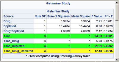
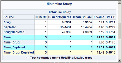
These next steps display the same table, but this time changing the background color for the entire row to highlight effects with p-values less than 0.001 and also those with p-values less than 0.01. The table is displayed three times. Output 20.7.6 displays the results by using bold green and yellow backgrounds and a bold font. Output 20.7.7 displays the results by using subtler cyan and yellow backgrounds and a bold font. Output 20.7.8 displays the results by using very subtle cyan and gray backgrounds and a normal font. This control is provided by the CELLSTYLE statement in PROC TEMPLATE. You can do many things with the CELLSTYLE statement to enhance your output. Several more are shown in other examples in this chapter. These next steps create the custom template with varying colors and fonts and display the results by using PROC SGRENDER:
%macro hilight(c1,c2);
   proc template;
      define table CombinedTests;
         parent=Stat.GLM.Tests;

         header '#Histamine Study##';
         footer '#* - Test computed using Hotelling-Lawley trace';

         column Source DF SS MS FValue ProbF;

         cellstyle probf <= 0.001 as {background=&c1},
                   probf <= 0.01  as {background=&c2};

         define DF; format=bestd3.; end;
         define SS;
            parent=Stat.GLM.SS
            choose_format=max format_width=7;
            translate _val_ = . into '  *';
         end;
         define MS;
            parent=Stat.GLM.MS
            choose_format=max format_width=7;
            translate _val_ = . into '  *';
         end;
      end;
   run;

   proc sgrender data=HistTests template=CombinedTests;
   run;
%mend;

title2;
ods _all_ close;
ods html style=HTMLBlue;

%hilight(CX22FF22 fontweight=bold, CXFFFF22 fontweight=bold)
%hilight(CXAAFFFF fontweight=bold, CXFFFFDD fontweight=bold)
%hilight(CXEEFAFA, CXEEEEEE)

ods html close;
ods listing;

All colors are specified in values of the form CXrrggbb, where the last six characters specify RGB (red, green, blue) values on the hexadecimal scale of 00 to FF (or 0 to 255 base 10). You can run the following step to see the correspondence between the integer and HEX formatting of values in the range 0 to 255:
data _null_;
   do color = 0 to 255;
      put color 3. +1 color hex2.;
   end;
run;
The results of this step are not shown. Hexadecimal values 0 through F represent the numbers 0 to 15. A hex value xy can be converted to an integer as follows: ![]() . For example, BC is
. For example, BC is ![]() . Common colors are CXFF0000 (red), CX00FF00 (green), CX0000FF (blue), CXFFFF00 (yellow, a mix of red and green), CXFF00FF
(magenta, a mix of red and blue), CX00FFFF (cyan, a mix of green and blue), CXFFFFFF (white, a mix of red, green, and blue),
CX000000 (black, no color), CXDDDDDD (very light gray), CX222222 (very dark gray), and so on. Colors become lighter as the
RGB values increase and darker as they decrease. For example, cyan (CX00FFFF) can be lightened by increasing the red component
from 00 to FF until eventually it becomes indistinguishable from white. It can be darkened by jointly decreasing the green
and blue values until it becomes indistinguishable from black.
. Common colors are CXFF0000 (red), CX00FF00 (green), CX0000FF (blue), CXFFFF00 (yellow, a mix of red and green), CXFF00FF
(magenta, a mix of red and blue), CX00FFFF (cyan, a mix of green and blue), CXFFFFFF (white, a mix of red, green, and blue),
CX000000 (black, no color), CXDDDDDD (very light gray), CX222222 (very dark gray), and so on. Colors become lighter as the
RGB values increase and darker as they decrease. For example, cyan (CX00FFFF) can be lightened by increasing the red component
from 00 to FF until eventually it becomes indistinguishable from white. It can be darkened by jointly decreasing the green
and blue values until it becomes indistinguishable from black.
The three CELLSTYLE statements that set the colors after the macro variables are substituted are as follows:
cellstyle probf <= 0.001 as {background=CX22FF22 fontweight=bold},
          probf <= 0.01  as {background=CXFFFF22 fontweight=bold};
cellstyle probf <= 0.001 as {background=CXAAFFFF fontweight=bold},
          probf <= 0.01  as {background=CXFFFFDD fontweight=bold};
cellstyle probf <= 0.001 as {background=CXEEFAFA},
          probf <= 0.01  as {background=CXEEEEEE};
The first color, CX22FF22, for the smallest p-values in the first table is a bold green color. The first table uses almost pure green and pure yellow, but a little red and blue are added to slightly lighten the colors. The second table uses a cyan and yellow that are very light due to the addition of AA (170) red and DD (221) blue, respectively. The third table uses a cyan that is not much different from light gray, and a light gray that is not much different from white.