The NPAR1WAY Procedure

This example illustrates how you can use PROC NPAR1WAY to perform a one-way nonparametric analysis. The data from Halverson and Sherwood (1930) consist of weight gain measurements for five different levels of gossypol additive in animal feed. Gossypol is a substance contained in cottonseed shells, and these data were collected to study the effect of gossypol on animal nutrition.
The following DATA step statements create the SAS data set Gossypol:
data Gossypol;
   input Dose n;
   do i=1 to n;
      input Gain @@;
      output;
   end;
   datalines;
0 16
228 229 218 216 224 208 235 229 233 219 224 220 232 200 208 232
.04 11
186 229 220 208 228 198 222 273 216 198 213
.07 12
179 193 183 180 143 204 114 188 178 134 208 196
.10 17
130 87 135 116 118 165 151 59 126 64 78 94 150 160 122 110 178
.13 11
154 130 130 118 118 104 112 134 98 100 104
;
The data set Gossypol contains the variable Dose, which represents the amount of gossypol additive, and the variable Gain, which represents the weight gain.
Researchers are interested in whether there is a difference in weight gain among animals receiving the different dose levels of gossypol. The following statements invoke the NPAR1WAY procedure to perform a nonparametric analysis of this problem:
proc npar1way data=Gossypol;
   class Dose;
   var Gain;
run;
The variable Dose is the CLASS variable, and the VAR statement specifies the variable Gain is the response variable. The CLASS statement is required, and you must name only one CLASS variable. You can name one or
more analysis variables in the VAR statement. If you omit the VAR statement, PROC NPAR1WAY analyzes all numeric variables
in the data set except for the CLASS variable, the FREQ variable, and the BY variables.
When no analysis options are specified in the PROC NPAR1WAY statement, the ANOVA, WILCOXON, MEDIAN, VW, SAVAGE, and EDF options are invoked by default. The tables in the following figures show the results of these analyses.
The tables in Figure 71.1 are produced by the ANOVA option. For each level of the CLASS variable Dose, PROC NPAR1WAY displays the number of observations and the mean of the analysis variable Gain. PROC NPAR1WAY displays a standard analysis of variance on the raw data. This gives the same results as the GLM and ANOVA
procedures. The p-value for the F test is <0.0001, which indicates that Dose accounts for a significant portion of the variability of the dependent variable Gain.
The WILCOXON option produces the output in Figure 71.2. PROC NPAR1WAY first provides a summary of the Wilcoxon scores for the analysis variable Gain by class level. For each level of the CLASS variable Dose, PROC NPAR1WAY displays the following information: number of observations, sum of the Wilcoxon scores, expected sum under
the null hypothesis of no difference among class levels, standard deviation under the null hypothesis, and mean score.
Next PROC NPAR1WAY displays the one-way ANOVA statistic, which for Wilcoxon scores is known as the Kruskal-Wallis test. The
statistic equals 52.6656, with four degrees of freedom, which is the number of class levels minus one. The p-value (probability of a larger statistic under the null hypothesis) is <0.0001. This leads to rejection of the null hypothesis
that there is no difference in location for Gain among the levels of Dose. This p-value is asymptotic, computed from the asymptotic chi-square distribution of the test statistic. For certain data sets it
might also be useful to compute the exact p-value—for example, for small data sets or for data sets that are sparse, skewed, or heavily tied. You can use the EXACT statement
to request exact p-values for any of the location or scale tests available in PROC NPAR1WAY.
Figure 71.2: Wilcoxon Score Analysis
| Wilcoxon Scores (Rank Sums) for Variable Gain Classified by Variable Dose |
|||||
|---|---|---|---|---|---|
| Dose | N | Sum of Scores |
Expected Under H0 |
Std Dev Under H0 |
Mean Score |
| 0 | 16 | 890.50 | 544.0 | 67.978966 | 55.656250 |
| 0.04 | 11 | 555.00 | 374.0 | 59.063588 | 50.454545 |
| 0.07 | 12 | 395.50 | 408.0 | 61.136622 | 32.958333 |
| 0.1 | 17 | 275.50 | 578.0 | 69.380741 | 16.205882 |
| 0.13 | 11 | 161.50 | 374.0 | 59.063588 | 14.681818 |
| Average scores were used for ties. | |||||
Figure 71.3 through Figure 71.5 display the analyses produced by the MEDIAN, VW, and SAVAGE options. For each score type, PROC NPAR1WAY provides a summary of scores and the one-way ANOVA statistic, as previously described for Wilcoxon scores. Other score types available in PROC NPAR1WAY are Siegel-Tukey, Ansari-Bradley, Klotz, and Mood, which can be used to test for scale differences. Conover scores can be used to test for differences in both location and scale. Additionally, you can specify the SCORES=DATA option, which uses the input data as scores. This option gives you the flexibility to construct any scores for your data with the DATA step and then analyze these scores with PROC NPAR1WAY.
Figure 71.3: Median Score Analysis
| Median Scores (Number of Points Above Median) for Variable Gain Classified by Variable Dose |
|||||
|---|---|---|---|---|---|
| Dose | N | Sum of Scores |
Expected Under H0 |
Std Dev Under H0 |
Mean Score |
| 0 | 16 | 16.0 | 7.880597 | 1.757902 | 1.00 |
| 0.04 | 11 | 11.0 | 5.417910 | 1.527355 | 1.00 |
| 0.07 | 12 | 6.0 | 5.910448 | 1.580963 | 0.50 |
| 0.1 | 17 | 0.0 | 8.373134 | 1.794152 | 0.00 |
| 0.13 | 11 | 0.0 | 5.417910 | 1.527355 | 0.00 |
| Average scores were used for ties. | |||||
Figure 71.4: Van der Waerden (Normal) Score Analysis
| Van der Waerden Scores (Normal) for Variable Gain Classified by Variable Dose |
|||||
|---|---|---|---|---|---|
| Dose | N | Sum of Scores |
Expected Under H0 |
Std Dev Under H0 |
Mean Score |
| 0 | 16 | 16.116474 | 0.0 | 3.325957 | 1.007280 |
| 0.04 | 11 | 8.340899 | 0.0 | 2.889761 | 0.758264 |
| 0.07 | 12 | -0.576674 | 0.0 | 2.991186 | -0.048056 |
| 0.1 | 17 | -14.688921 | 0.0 | 3.394540 | -0.864054 |
| 0.13 | 11 | -9.191777 | 0.0 | 2.889761 | -0.835616 |
| Average scores were used for ties. | |||||
Figure 71.5: Savage Score Analysis
| Savage Scores (Exponential) for Variable Gain Classified by Variable Dose |
|||||
|---|---|---|---|---|---|
| Dose | N | Sum of Scores |
Expected Under H0 |
Std Dev Under H0 |
Mean Score |
| 0 | 16 | 16.074391 | 0.0 | 3.385275 | 1.004649 |
| 0.04 | 11 | 7.693099 | 0.0 | 2.941300 | 0.699373 |
| 0.07 | 12 | -3.584958 | 0.0 | 3.044534 | -0.298746 |
| 0.1 | 17 | -11.979488 | 0.0 | 3.455082 | -0.704676 |
| 0.13 | 11 | -8.203044 | 0.0 | 2.941300 | -0.745731 |
| Average scores were used for ties. | |||||
The tables in Figure 71.6 display the empirical distribution function statistics, comparing the distribution of Gain for the different levels of Dose. These tables are produced by the EDF option, and they include Kolmogorov-Smirnov statistics and Cramér–von Mises statistics.
Figure 71.6: Empirical Distribution Function Analysis
| Kolmogorov-Smirnov Test for Variable Gain Classified by Variable Dose |
|||
|---|---|---|---|
| Dose | N | EDF at Maximum |
Deviation from Mean at Maximum |
| 0 | 16 | 0.000000 | -1.910448 |
| 0.04 | 11 | 0.000000 | -1.584060 |
| 0.07 | 12 | 0.333333 | -0.499796 |
| 0.1 | 17 | 1.000000 | 2.153861 |
| 0.13 | 11 | 1.000000 | 1.732565 |
| Total | 67 | 0.477612 | |
| Maximum Deviation Occurred at Observation 36 | |||
| Value of Gain at Maximum = 178.0 | |||
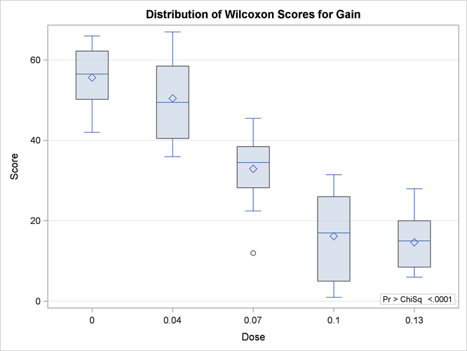
PROC NPAR1WAY uses ODS Graphics to create graphs as part of its output. The following statements produce a box plot of Wilcoxon
scores for Gain classified by Dose. ODS Graphics must be enabled before producing graphs.
ods graphics on;
proc npar1way data=Gossypol plots(only)=wilcoxonboxplot;
   class Dose;
   var Gain;
run;
ods graphics off;
Figure 71.7 displays the box plot of Wilcoxon scores. This graph corresponds to the Wilcoxon scores analysis shown in Figure 71.2. To remove the p-value from the box plot display, you can specify the NOSTATS plot option in parentheses following the WILCOXONBOXPLOT option.
Box plots are available for all PROC NPAR1WAY score types except median scores, which are displayed in a stacked bar chart. If ODS Graphics is enabled but you do not specify the PLOTS= option, PROC NPAR1WAY produces all plots that are associated with the analyses that you request.
In the preceding example, the CLASS variable Dose has five levels, and the analyses examine possible differences among these five levels (samples). The following statements
invoke the NPAR1WAY procedure to perform a nonparametric analysis of the two lowest levels of Dose:
proc npar1way data=Gossypol;
   where Dose <= .04;
   class Dose;
   var Gain;
run;
The tables in the following figures show the results of this two-sample analysis. The tables in Figure 71.8 are produced by the ANOVA option.
Figure 71.9 displays the output produced by the WILCOXON option. PROC NPAR1WAY provides a summary of the Wilcoxon scores for the analysis
variable Gain for each of the two class levels. Since there are only two levels, PROC NPAR1WAY displays the two-sample test, based on the
simple linear rank statistic with Wilcoxon scores. The normal approximation includes a continuity correction. To remove the
continuity correction, you can specify the CORRECT=NO option. PROC NPAR1WAY also gives a t approximation for the Wilcoxon two-sample test. Like the multisample analysis, PROC NPAR1WAY computes a one-way ANOVA statistic,
which for Wilcoxon scores is known as the Kruskal-Wallis test. All these p-values show no difference in Gain for the two Dose levels at the 0.05 level of significance.
Figure 71.10 through Figure 71.12 display the two-sample analyses produced by the MEDIAN, VW, and SAVAGE options.
The tables in Figure 71.13 display the empirical distribution function statistics, comparing the distribution of Gain for the two levels of Dose. The p-value for the Kolmogorov-Smirnov two-sample test is 0.6199, which indicates no rejection of the null hypothesis that the
Gain distributions are identical for the two levels of Dose.