The NLIN Procedure
- Overview
-
Getting Started

-
Syntax
-
DetailsAutomatic DerivativesMeasures of Nonlinearity, Diagnostics and InferenceMissing ValuesSpecial VariablesTroubleshootingComputational MethodsOutput Data SetsConfidence IntervalsCovariance Matrix of Parameter EstimatesConvergence MeasuresDisplayed OutputIncompatibilities with SAS 6.11 and Earlier Versions of PROC NLINODS Table NamesODS Graphics
-
Examples
- References
This example, which uses a model from Clarke (1987), shows why it is difficult to intuitively reason about the characteristics of the parameters that occur in a nonlinear model. As a consequence, the example demonstrates the indispensability of parameter profiling and confidence curves to identify the nonlinear characteristics of model parameters. The parameter profiling is also augmented with a plot that shows the influence of each observation on the parameter estimates. Furthermore, the BOOTSTRAP statement in PROC NLIN is invoked in order to study the sampling distribution of parameter estimates and make more accurate statistical inferences.
The model takes the form
The data set in this example is from Clarke (1987). The following DATA step creates this data set:
data clarke1987a;
   input  x y;
   datalines;
1    3.183
2    3.059
3    2.871
4    2.622
5    2.541
6    2.184
7    2.110
8    2.075
9    2.018
10   1.903
11   1.770
12   1.762
13   1.550
;
The model is fit by using the following statements in the NLIN procedure:
ods graphics on;
proc nlin data=clarke1987a plots(stats=none)=diagnostics;
   parms theta1=-0.15
         theta2=2.0
         theta3=0.80;
   profile theta1 theta3 / range = -6 to 2 by 0.2 all;
   bootstrap / nsamples = 2000 seed=123 bootplots bootci bootcov;
   model y = theta3 + theta2*exp(theta1*x);
run;
ods graphics off;
Output 69.7.1: Parameter Estimates and Bootstrap Estimate of the Covariance Matrix
| Parameter | Estimate | Approx Std Error |
Approximate 95% Confidence Limits |
Bootstrap Std Dev |
Bootstrap Bias-Corrected 95% Confidence Limits |
||
|---|---|---|---|---|---|---|---|
| theta1 | -0.1031 | 0.0255 | -0.1599 | -0.0462 | 0.0253 | -0.1505 | -0.0531 |
| theta2 | 2.5190 | 0.2658 | 1.9268 | 3.1112 | 0.4450 | 2.1716 | 3.5325 |
| theta3 | 0.9631 | 0.3216 | 0.2466 | 1.6797 | 0.4907 | -0.2565 | 1.3697 |
By default, the BOOTCI
option in the BOOTSTRAP
statement adds a column that contains the bias-corrected bootstrap confidence limits to the "Parameter Estimates" table (Output 69.7.1). The BOOTCOV
option produces the "Bootstrap Covariance Matrix" table (Output 69.7.1). The discrepancy between the Wald-based confidence limits and the bias-corrected bootstrap confidence limits is much greater
for ![]() than for
than for ![]() . The profile t plot, confidence curve, and histograms of the bootstrap estimates show why this is the case.
. The profile t plot, confidence curve, and histograms of the bootstrap estimates show why this is the case.
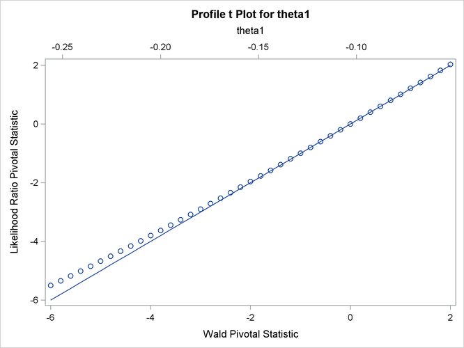
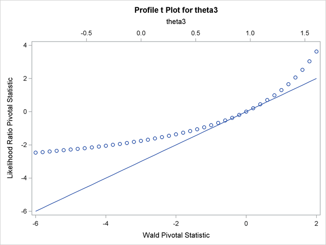
The profile t plot for parameter ![]() in Output 69.7.3 shows a definite deviation from the linear reference line that has a slope of 1 and passes through the origin. Hence, Wald-based
inference for
in Output 69.7.3 shows a definite deviation from the linear reference line that has a slope of 1 and passes through the origin. Hence, Wald-based
inference for ![]() is not appropriate. In contrast, the profile t plot for parameter
is not appropriate. In contrast, the profile t plot for parameter ![]() in Output 69.7.2 shows that Wald-based inference for
in Output 69.7.2 shows that Wald-based inference for ![]() might be sufficient.
might be sufficient.
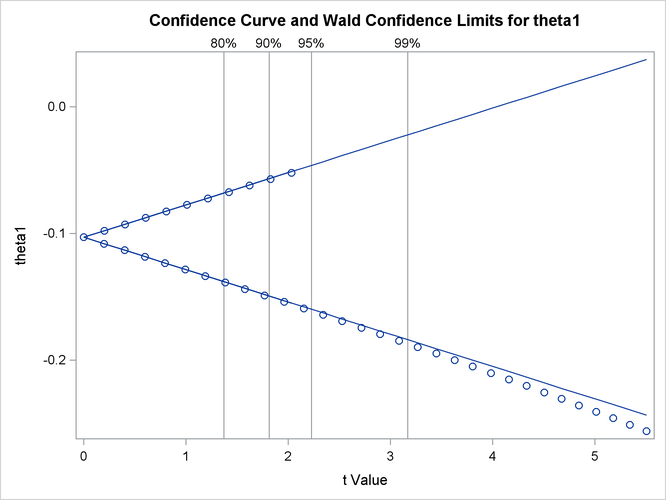
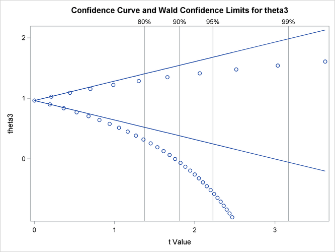
Output 69.7.4 and Output 69.7.5 show the confidence curves for ![]() and
and ![]() , respectively. For
, respectively. For ![]() , you can see a significant difference between the Wald-based confidence interval and the corresponding likelihood-based interval.
In such cases, the likelihood-based intervals are preferred because their coverage rate is much closer to the nominal values
than the coverage rate of the Wald-based intervals (Donaldson and Schnabel, 1987; Cook and Weisberg, 1990).
, you can see a significant difference between the Wald-based confidence interval and the corresponding likelihood-based interval.
In such cases, the likelihood-based intervals are preferred because their coverage rate is much closer to the nominal values
than the coverage rate of the Wald-based intervals (Donaldson and Schnabel, 1987; Cook and Weisberg, 1990).
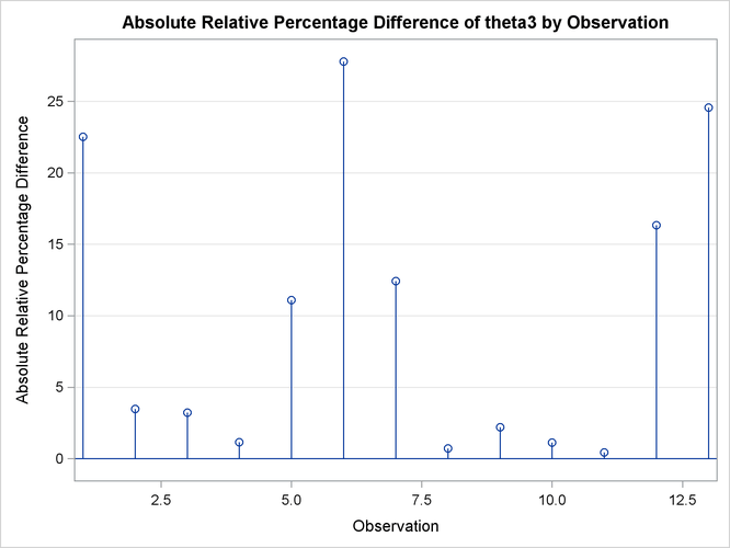
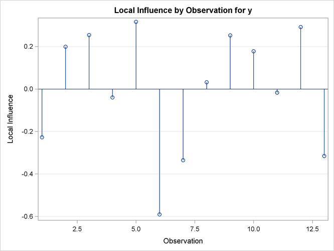
Output 69.7.6 depicts the influence of each observation on the value of ![]() . Observations 6 and 13 have the most influence on the value of this parameter. The plot is generated using the leave-one-out
method and should be contrasted with the local influence plot in Output 69.7.7, which is based on assessing the influence of an additive perturbation of the response variable.
. Observations 6 and 13 have the most influence on the value of this parameter. The plot is generated using the leave-one-out
method and should be contrasted with the local influence plot in Output 69.7.7, which is based on assessing the influence of an additive perturbation of the response variable.
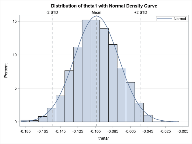
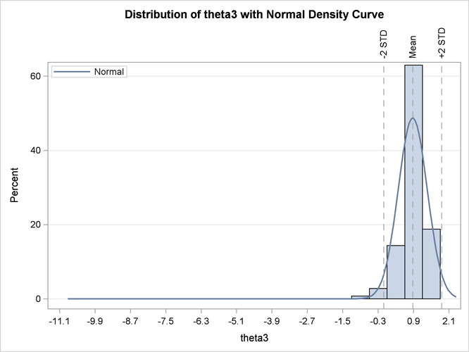
Output 69.7.8 and Output 69.7.9 are histograms that show the distribution of the bootstrap parameter estimates for ![]() and
and ![]() , respectively. These histograms complement the information that is obtained about
, respectively. These histograms complement the information that is obtained about ![]() and
and ![]() from the profile t plots. Specifically, they show that the bootstrap parameter estimate of
from the profile t plots. Specifically, they show that the bootstrap parameter estimate of ![]() has a distribution close to normal, whereas that of
has a distribution close to normal, whereas that of ![]() has a distribution that deviates significantly from normal. Again, this leads to the conclusion that inferences based on
linear approximations, such as Wald-based confidence intervals, work better for
has a distribution that deviates significantly from normal. Again, this leads to the conclusion that inferences based on
linear approximations, such as Wald-based confidence intervals, work better for ![]() than for
than for ![]() .
.
Finally, this example shows that the adequacy of a linear approximation with regard to a certain parameter cannot be inferred
directly from the model. If it could, then ![]() , which enters the model linearly, would have a completely linear behavior, whereas
, which enters the model linearly, would have a completely linear behavior, whereas ![]() would have a highly nonlinear behavior. However, the diagnostics that are based on the profile t plot and confidence curves, and the histograms of the bootstrap parameter estimates, show that the opposite holds. For a
detailed discussion about this issue, see Cook and Weisberg (1990).
would have a highly nonlinear behavior. However, the diagnostics that are based on the profile t plot and confidence curves, and the histograms of the bootstrap parameter estimates, show that the opposite holds. For a
detailed discussion about this issue, see Cook and Weisberg (1990).