The LOESS Procedure
-
Overview

-
Getting Started
-
Syntax
-
DetailsMissing ValuesOutput Data SetsData ScalingDirect versus Interpolated Fittingk-d Trees and BlendingLocal WeightingIterative ReweightingSpecifying the Local PolynomialsSmoothing MatrixModel Degrees of FreedomStatistical Inference and Lookup Degrees of FreedomAutomatic Smoothing Parameter SelectionSparse and Approximate Degrees of Freedom ComputationScoring Data SetsODS Table NamesODS Graphics
-
Examples
- References
The following data set records the results of an experiment to determine how the yield of a chemical reaction varies with temperature and amount of a catalyst used.
data Experiment;
   input Temperature Catalyst MeasuredYield;
   if ranuni(1) < 0.1
      then CorruptedYield = MeasuredYield + 10 * ranuni(1);
      else CorruptedYield = MeasuredYield;
   datalines;
 80    0.000     6.85601
 80    0.002     7.26355
 80    0.004     7.41448
 80    0.006     7.82640

   ... more lines ...

140    0.078     5.20562
140    0.080     5.49371
;
The aim of this example is to show how you can use PROC LOESS for robust fitting in the presence of outliers. To simulate
an intermittent equipment malfunction, the variable CorruptedYield is the same as the variable MeasuredYield except for about 10% of the observations where an offset has been added. This example shows how you can use PROC LOESS obtain
a fit for CorruptedYield that is close to the fit you obtain for MeasuredYield.
The following statements produce a scatter plot of Temperature by Catalyst where the observations are colored by CorruptedYield:
proc template;
   define statgraph gradientScatter;
      beginGraph;
         layout overlay;
            scatterPlot x=Catalyst y=Temperature /
                markercolorgradient = CorruptedYield
                markerattrs         = (symbol=circleFilled)
                colormodel          =  ThreeColorRamp
                name                =  "Yield";

            scatterPlot x=Catalyst y=Temperature /
                markerattrs         = (symbol=circle);

            continuousLegend "Yield" / title= "CorruptedYield";
         endlayout;
      endgraph;
   end;
run;

proc sgrender data=Experiment template=gradientScatter;
run;
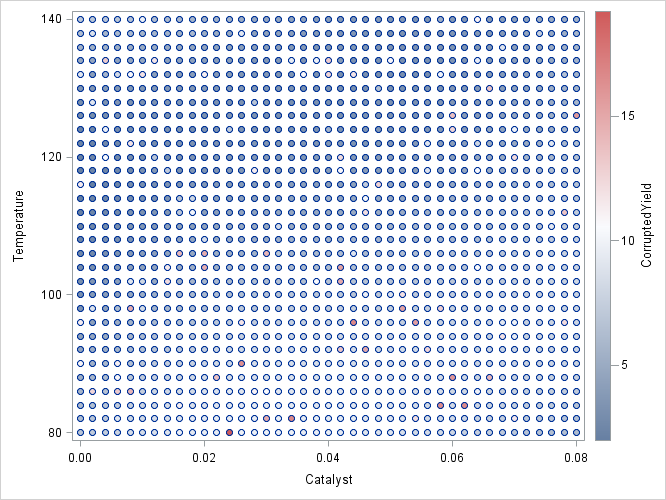
Output 59.3.1 shows a scatter plot of the data where the observations are shaded by the value of CorruptedYield. The darkly shaded points that are surrounded by lightly shaded points are points where the simulated incorrect measurements
occur.
The following code fits a loess model to the measured data:
ods graphics on;

proc loess data=Experiment;
   model MeasuredYield = Temperature Catalyst / scale=sd(0.1);
run;
The SCALE=SD(0.1) option in the MODEL
statement specifies that the independent variables in the model are to be divided by their respective 10% trimmed standard
deviations before the fitted model is computed. This is appropriate because the independent variables Temperature and Catalyst are not similarly scaled. The "Scale Details" table in Output 59.3.2 displays the details of ranges of the regressors and the scale factors applied to each regressor.
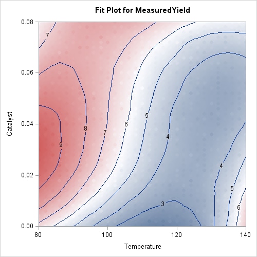
Output 59.3.3 displays the loess fit. Because the fitted surface is a good fit of the observed data, the observations on this plot are not clearly distinguishable from the fitted surface. The results are dramatically different when the outliers are included. The following statements fit a loess model to the corrupted response, using the same smoothing parameter that was selected for the measured response.
proc loess data=Experiment;
   model CorruptedYield = Temperature Catalyst /
                 scale=sd(0.1) smooth=0.018;
run;
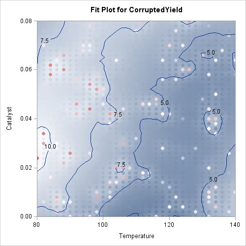
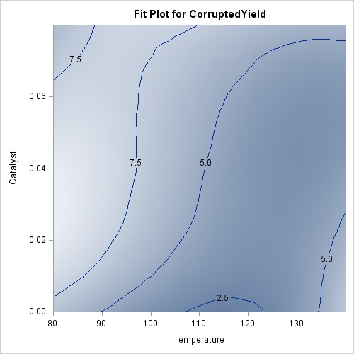
Output 59.3.4 displays the loess fit. The fit is pulled upward in the neighborhoods of these outliers. If you use a larger smoothing parameter value, then these local perturbations in the fit get smoothed out, but at the expense of smoothing away the information in the underlying measured response. In such cases a robust fitting method is indicated. The following statements show how you do this:
proc loess data=Experiment;
   model CorruptedYield = Temperature Catalyst /
                             scale  = sd(0.1)
                             smooth = 0.018
                             iterations=4;
run;
The ITERATIONS=4 option in the MODEL statement requests the initial loess fit followed by three iteratively reweighted iterations.
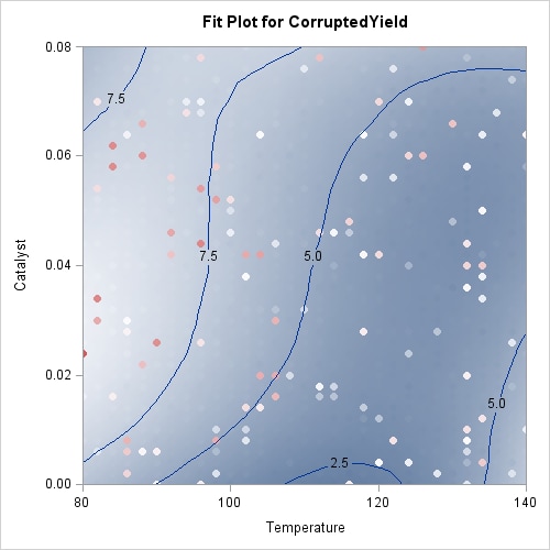
You can see the impact of the robust fitting by comparing the robust fit shown in Output 59.3.5 with the nonrobust fit in Output 59.3.4. In the robust fit you see that the local perturbations caused by the outliers have been eliminated as these the outlying observations get down-weighted during the robustness iterations. By comparing the labeled contours on the fit plot for the uncorrupted response shown in Output 59.3.3 with the labeled contours for the corrupted response shown in Output 59.3.4, you can see that the robust fit has produced a reasonable fit for the underlying measured data. The color gradient in Output 59.3.5 is chosen to accommodate the outliers that are present in the observed data, and so you cannot easily compare the color gradient in this plot with that in Output 59.3.3. The following statements repeat the robust analysis with an option added to suppress the display of the observations on the fit plot:
proc loess data=Experiment plots=contourFit(obs=none);
   model CorruptedYield = Temperature Catalyst /
                            scale  = sd(0.1)
                            smooth = 0.018
                            iterations=4;
run;

ods graphics off;
Output 59.3.6 shows the robust fit with the observations suppressed. The range of the fitted surface values in this plot is similar to the range in Output 59.3.3. By comparing this contour plot with the contour plot in Output 59.3.3, you clearly see that the robust loess fit has successfully modeled the underlying surface despite the presence of the outliers.