The LOESS Procedure
-
Overview

-
Getting Started
-
Syntax
-
DetailsMissing ValuesOutput Data SetsData ScalingDirect versus Interpolated Fittingk-d Trees and BlendingLocal WeightingIterative ReweightingSpecifying the Local PolynomialsSmoothing MatrixModel Degrees of FreedomStatistical Inference and Lookup Degrees of FreedomAutomatic Smoothing Parameter SelectionSparse and Approximate Degrees of Freedom ComputationScoring Data SetsODS Table NamesODS Graphics
-
Examples
- References
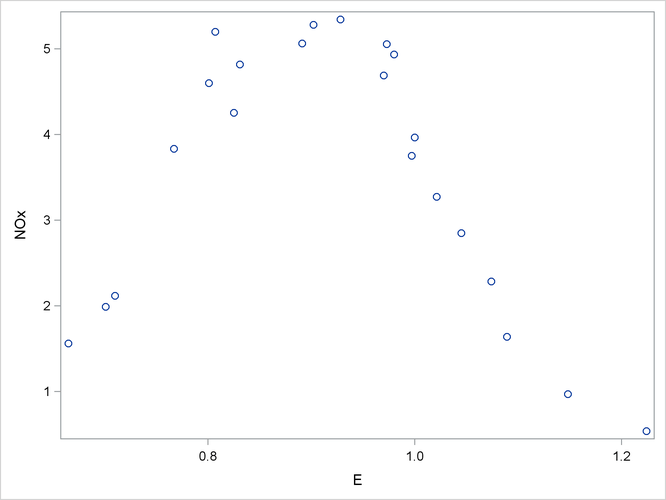
Investigators studied the exhaust emissions of a one-cylinder engine (Brinkman, 1981). The SAS data set Gas contains the results data. The dependent variable, NOx, measures the concentration, in micrograms per joule, of nitric oxide and nitrogen dioxide normalized by the amount of work
of the engine. The independent variable, E, is a measure of the richness of the air and fuel mixture.
data Gas;
   input NOx E @@;
   format NOx f3.1;
   format E f3.1;
   datalines;
4.818  0.831   2.849  1.045
3.275  1.021   4.691  0.97
4.255  0.825   5.064  0.891
2.118  0.71    4.602  0.801
2.286  1.074   0.97   1.148
3.965  1       5.344  0.928
3.834  0.767   1.99   0.701
5.199  0.807   5.283  0.902
3.752  0.997   0.537  1.224
1.64   1.089   5.055  0.973
4.937  0.98    1.561  0.665
;
The following PROC SGPLOT statements produce the simple scatter plot of these data displayed in Output 59.1.1.
proc sgplot data=Gas;
   scatter x=E y=NOx;
run;
The following statements fit two loess models for these data. Because this is a small data set, it is reasonable to do direct fitting at every data point. As there is substantial curvature in the data, quadratic local polynomials are used. An ODS OUTPUT statement creates two output data sets containing the "Output Statistics" and "Fit Summary" tables.
ods graphics on;

proc loess data=Gas;
   ods output OutputStatistics = GasFit
              FitSummary=Summary;
   model NOx = E / degree=2 select=AICC(steps) smooth = 0.6 1.0
                   direct alpha=.01 all details;
run;

ods graphics off;
Output 59.1.2: Fit Summary Table
| Fit Summary | |
|---|---|
| Fit Method | Direct |
| Number of Observations | 22 |
| Degree of Local Polynomials | 2 |
| Smoothing Parameter | 0.60000 |
| Points in Local Neighborhood | 13 |
| Residual Sum of Squares | 1.71852 |
| Trace[L] | 6.42184 |
| GCV | 0.00708 |
| AICC | -0.45637 |
| AICC1 | -9.39715 |
| Delta1 | 15.12582 |
| Delta2 | 14.73089 |
| Equivalent Number of Parameters | 5.96950 |
| Lookup Degrees of Freedom | 15.53133 |
| Residual Standard Error | 0.33707 |
The "Fit Summary" table for smoothing parameter value 0.6, shown in Output 59.1.2, records the fitting parameters specified and some overall fit statistics. See the section Smoothing Matrix for a definition of the smoothing matrix ![]() , and the sections Model Degrees of Freedom and Statistical Inference and Lookup Degrees of Freedom for definitions of the statistics that appear this table.
, and the sections Model Degrees of Freedom and Statistical Inference and Lookup Degrees of Freedom for definitions of the statistics that appear this table.
The "Output Statistics" table for smoothing parameter value 0.6 is shown in Output 59.1.3. Note that, because the ALL option is specified in the MODEL statement, this table includes all the relevant optional columns. Furthermore, because the ALPHA=0.01 option is specified in the MODEL statement, the confidence limits in this table are 99% limits.
Output 59.1.3: Output Statistics Table
| Output Statistics | ||||||||
|---|---|---|---|---|---|---|---|---|
| Obs | E | NOx | Predicted NOx | Estimated Prediction Std Deviation |
Residual | t Value | 99% Confidence Limits | |
| 1 | 0.8 | 4.8 | 4.87377 | 0.15528 | -0.05577 | -0.36 | 4.41841 | 5.32912 |
| 2 | 1.0 | 2.8 | 2.81984 | 0.15380 | 0.02916 | 0.19 | 2.36883 | 3.27085 |
| 3 | 1.0 | 3.3 | 3.48153 | 0.15187 | -0.20653 | -1.36 | 3.03617 | 3.92689 |
| 4 | 1.0 | 4.7 | 4.73249 | 0.13923 | -0.04149 | -0.30 | 4.32419 | 5.14079 |
| 5 | 0.8 | 4.3 | 4.82305 | 0.15278 | -0.56805 | -3.72 | 4.37503 | 5.27107 |
| 6 | 0.9 | 5.1 | 5.18561 | 0.19337 | -0.12161 | -0.63 | 4.61855 | 5.75266 |
| 7 | 0.7 | 2.1 | 2.51120 | 0.15528 | -0.39320 | -2.53 | 2.05585 | 2.96655 |
| 8 | 0.8 | 4.6 | 4.48267 | 0.15285 | 0.11933 | 0.78 | 4.03444 | 4.93089 |
| 9 | 1.1 | 2.3 | 2.12619 | 0.16683 | 0.15981 | 0.96 | 1.63697 | 2.61541 |
| 10 | 1.1 | 1.0 | 0.97120 | 0.18134 | -0.00120 | -0.01 | 0.43942 | 1.50298 |
| 11 | 1.0 | 4.0 | 4.09987 | 0.13477 | -0.13487 | -1.00 | 3.70467 | 4.49507 |
| 12 | 0.9 | 5.3 | 5.31258 | 0.17283 | 0.03142 | 0.18 | 4.80576 | 5.81940 |
| 13 | 0.8 | 3.8 | 3.84572 | 0.14929 | -0.01172 | -0.08 | 3.40794 | 4.28350 |
| 14 | 0.7 | 2.0 | 2.26578 | 0.16712 | -0.27578 | -1.65 | 1.77571 | 2.75584 |
| 15 | 0.8 | 5.2 | 4.58394 | 0.15363 | 0.61506 | 4.00 | 4.13342 | 5.03445 |
| 16 | 0.9 | 5.3 | 5.24741 | 0.19319 | 0.03559 | 0.18 | 4.68089 | 5.81393 |
| 17 | 1.0 | 3.8 | 4.16979 | 0.13478 | -0.41779 | -3.10 | 3.77457 | 4.56502 |
| 18 | 1.2 | 0.5 | 0.53059 | 0.32170 | 0.00641 | 0.02 | -0.41278 | 1.47397 |
| 19 | 1.1 | 1.6 | 1.83157 | 0.17127 | -0.19157 | -1.12 | 1.32933 | 2.33380 |
| 20 | 1.0 | 5.1 | 4.66733 | 0.13735 | 0.38767 | 2.82 | 4.26456 | 5.07010 |
| 21 | 1.0 | 4.9 | 4.52385 | 0.13556 | 0.41315 | 3.05 | 4.12632 | 4.92139 |
| 22 | 0.7 | 1.6 | 1.19888 | 0.26774 | 0.36212 | 1.35 | 0.41375 | 1.98401 |
The combination of the options SELECT=AICC and SMOOTH=0.6 1 in the MODEL statement specifies that PROC LOESS fit models with smoothing parameters of 0.6 and 1 and select the model that yields the smaller value of the AICC statistic. The "Smoothing Criterion" shown in Output 59.1.4 shows that PROC LOESS selects the model with smoothing parameter value 0.6 as it yields the smaller value of the AICC statistic.
With ODS Graphics enabled, PROC LOESS produces a panel of fit plots whenever you specify the SMOOTH= option in the MODEL statement. These fit plots include confidence limits if you additionally specify the CLM option in the MODEL statement.
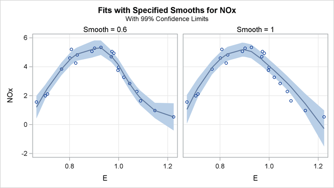
Output 59.1.5 shows the "Fit Panel" that displays the fitted models with 99% confidence limits overlaid on scatter plots of the data.
Based on the AICC criterion, the model with smoothing parameter 0.6 is preferred. You can address the question of whether the differences between these models are significant using analysis of variance. You do this by using the model with smoothing parameter value 1 as the null model.
The statistic
has a distribution that is well approximated by an F distribution with
numerator degrees of freedom and ![]() denominator degrees of freedom (Cleveland and Grosse, 1991). Here quantities with superscript n refer to the null model, rss is the residual sum of squares, and
denominator degrees of freedom (Cleveland and Grosse, 1991). Here quantities with superscript n refer to the null model, rss is the residual sum of squares, and ![]() ,
, ![]() , and
, and ![]() are defined in the section Statistical Inference and Lookup Degrees of Freedom.
are defined in the section Statistical Inference and Lookup Degrees of Freedom.
The "Fit Summary" tables contain the information needed to carry out such an analysis. These tables have been captured in
the output data set named Summary by using an ODS OUTPUT statement. The following statements extract the relevant information from this data set and carry
out the analysis of variance:
data h0 h1;
   set Summary(keep=SmoothingParameter Label1 nValue1
               where=(Label1 in ('Residual Sum of Squares','Delta1',
                      'Delta2','Lookup Degrees of Freedom')));
   if SmoothingParameter = 1 then output h0;
   else output h1;
run;

proc transpose data=h0(drop=SmoothingParameter Label1) out=h0;
run;

data h0(drop=_NAME_);
   set h0;
   rename Col1 = RSSNull
          Col2 = delta1Null
          Col3 = delta2Null;
run;

proc transpose data=h1(drop=SmoothingParameter Label1) out=h1;
run;

data h1(drop=_NAME_);
   set h1;
   rename Col1 = RSS     Col2 = delta1
          Col3 = delta2  Col4 = rho;
run;

data ftest;
   merge h0 h1;
   nu = (delta1Null - delta1)**2 / (delta2Null - delta2);
   Numerator = (RSSNull - RSS)/(delta1Null - delta1);
   Denominator = RSS/delta1;
   FValue = Numerator / Denominator;
   PValue = 1 - ProbF(FValue, nu, rho);
   label nu     = 'Num DF'   rho    = 'Den DF'
         FValue = 'F Value'  PValue = 'Pr > F';
run;

proc print data=ftest label;
   var nu rho Numerator Denominator FValue PValue;
   format nu rho FValue 7.2 PValue 6.4;
run;
The results are shown in Output 59.1.6.
The small p-value confirms that the fit with smoothing parameter value 0.6 is significantly different from the loess model with smoothing parameter value 1.
Alternatively, you can use the OUTPUT statement to generate the statistics you want to include in the output data set. The
following statements produce essentially the same results as the ODS OUTPUT statement does, except all the statistics for
each of the two smoothing parameter values are included because the SELECT= option is not specified in the MODEL statement.
In addition, with the ROW option specified, the output data set is arranged in rowwise format which enables you to compare
statistics side-by-side for a sequence of smoothing values. The ALL option after the slash produces all the statistics (predicted
values, residual values, standard errors of the mean predicted values, t statistics, and the lower and upper parts of ![]() % confidence limits on the mean predicted value). All these requested statistics are given their respective default names
in the output data set except the predicted value. The P=PREDVAL option causes the name for the predicted value to start with
% confidence limits on the mean predicted value). All these requested statistics are given their respective default names
in the output data set except the predicted value. The P=PREDVAL option causes the name for the predicted value to start with
predval.
proc loess data=Gas;
   model NOx = E / degree=2 smooth = 0.6 1.0
                   direct alpha=.01;
   output out=GasFit p=predval /all row;
run;