The GLMSELECT Procedure
-
Overview

- Getting Started
-
Syntax
-
DetailsModel-Selection MethodsModel Selection IssuesCriteria Used in Model Selection MethodsCLASS Variable Parameterization and the SPLIT OptionMacro Variables Containing Selected ModelsUsing the STORE StatementBuilding the SSCP MatrixModel AveragingUsing Validation and Test DataCross ValidationExternal Cross ValidationScreeningDisplayed OutputODS Table NamesODS Graphics
-
Examples
- References
This example shows how to use the elastic net method for model selection and compares it with the LASSO method. The example also uses k-fold external cross validation as a criterion in the CHOOSE= option to choose the best model based on the penalized regression fit.
This example uses a microarray data set called the leukemia (LEU) data set (Golub et al., 1999), which is used in the paper by Zou and Hastie (2005) to demonstrate the performance of the elastic net method in comparison with that of LASSO. The LEU data set consists of
7,129 genes and 72 samples, and 38 samples are used as training samples. Among the 38 training samples, 27 are type 1 leukemia
(acute lymphoblastic leukemia) and 11 are type 2 leukemia (acute myeloid leukemia). The goal is to construct a diagnostic
rule based on the expression level of those 7,219 genes to predict the type of leukemia. The remaining 34 samples are used
as the validation data for picking the appropriate model or as the test data for testing the performance of the selected model.
The training and validation data sets are available from Sashelp.Leutrain and Sashelp.Leutest.
To have a basis for comparison, use the following statements to apply the LASSO method for model selection:
ods graphics on;
proc glmselect data=sashelp.Leutrain valdata=sashelp.Leutest
               plots=coefficients;
   model y = x1-x7129/
         selection=LASSO(steps=120  choose=validate);
run;
The details about the number of observations for training and validation data are given in Output 48.6.1 and Output 48.6.2, respectively.
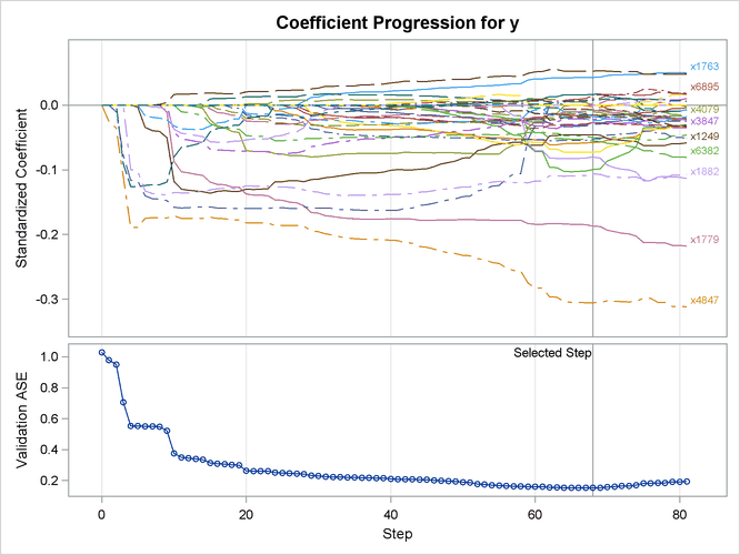
Output 48.6.3 shows the "LASSO Selection Summary" table. Although the STEPS= suboption of the SELECTION= option specifies that 120 steps of LASSO selection be performed, the LASSO method terminates at step 81 because the selected model is a perfect fit and the number of effects that can be selected by LASSO is bounded by the number of training samples. Note that a VALDATA= data set is named in the PROC GLMSELECT statement and that the minimum of the validation ASE occurs at step 68. Hence the model at this step is selected, resulting in 35 selected effects. Output 48.6.4 shows the standardized coefficients of all the effects selected at some step of the LASSO method, plotted as a function of the step number.
Output 48.6.3: LASSO Selection Summary Table
| The GLMSELECT Procedure |
| LASSO Selection Summary |
| Step | Effect Entered |
Effect Removed |
Number Effects In |
ASE | Validation ASE |
|---|---|---|---|---|---|
| 0 | Intercept | 1 | 0.8227 | 1.0287 | |
| 1 | x4847 | 2 | 0.7884 | 0.9787 | |
| 2 | x3320 | 3 | 0.7610 | 0.9507 | |
| 3 | x2020 | 4 | 0.4935 | 0.7061 | |
| 4 | x5039 | 5 | 0.2838 | 0.5527 | |
| 5 | x1249 | 6 | 0.2790 | 0.5518 | |
| 6 | x2242 | 7 | 0.2255 | 0.5513 | |
| . | . | . | |||
| . | . | . | |||
| . | . | . | |||
| 62 | x2534 | 35 | 0.0016 | 0.1554 | |
| 63 | x3320 | 34 | 0.0016 | 0.1557 | |
| 64 | x5631 | 35 | 0.0013 | 0.1532 | |
| 65 | x6021 | 34 | 0.0012 | 0.1534 | |
| 66 | x1745 | 33 | 0.0012 | 0.1535 | |
| 67 | x6376 | 34 | 0.0012 | 0.1535 | |
| 68 | x4831 | 35 | 0.0010 | 0.1531* | |
| 69 | x6184 | 34 | 0.0009 | 0.1539 | |
| 70 | x3820 | 35 | 0.0006 | 0.1588 | |
| 71 | x3171 | 36 | 0.0005 | 0.1615 | |
| 72 | x6376 | 35 | 0.0004 | 0.1640 | |
| 73 | x5142 | 36 | 0.0004 | 0.1659 | |
| 74 | x1745 | 37 | 0.0003 | 0.1688 | |
| 75 | x3605 | 38 | 0.0001 | 0.1821 | |
| 76 | x573 | 37 | 0.0001 | 0.1825 | |
| 77 | x3221 | 38 | 0.0001 | 0.1842 | |
| 78 | x1745 | 37 | 0.0001 | 0.1842 | |
| 79 | x6163 | 38 | 0.0000 | 0.1918 | |
| 80 | x4831 | 37 | 0.0000 | 0.1920 | |
| 81 | x1745 | 38 | 0.0000 | 0.1940 | |
| * Optimal Value of Criterion | |||||
As discussed earlier, the number of effects that can be selected by the LASSO method is upper-bounded by the number of training samples. However, this is not a restriction for the elastic net method, which incorporates an additional ridge regression penalty. You can use the following statements to apply the elastic net method for model selection:
proc glmselect data=sashelp.Leutrain valdata=sashelp.Leutest
               plots=coefficients;
   model y = x1-x7129/
         selection=elasticnet(steps=120 L2=0.001 choose=validate);
run;
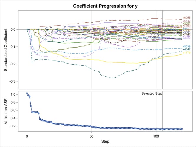
The L2= suboption of the SELECTION= option in the MODEL statement specifies the value of the ridge regression parameter. Output 48.6.5 shows the "Elastic Net Selection Summary" table. As in the example for LASSO, the STEPS= suboption of the SELECTION= option specifies that 120 steps of elastic net selection be performed. However, in contrast to the early termination in the LASSO method at step 81, the elastic net method runs until the specified 120 steps are performed. With the same VALDATA= data set named in the PROC GLMSELECT statement as in the LASSO example, the minimum of the validation ASE occurs at step 105, and hence the model at this step is selected, resulting in 54 selected effects. Compared with the LASSO method, the elastic net method can select more variables, and the number of selected variables is not restricted by the number of samples (38 for this example). Output 48.6.6 shows the standardized coefficients of all the effects that are selected at some step of the elastic net method, plotted as a function of the step number.
Output 48.6.5: Elastic Net Selection Summary Table
| The GLMSELECT Procedure |
| Elastic Net Selection Summary |
| Step | Effect Entered |
Effect Removed |
Number Effects In |
ASE | Validation ASE |
|---|---|---|---|---|---|
| 0 | Intercept | 1 | 0.8227 | 1.0287 | |
| 1 | x4847 | 2 | 0.7885 | 0.9790 | |
| 2 | x3320 | 3 | 0.7611 | 0.9510 | |
| 3 | x2020 | 4 | 0.4939 | 0.7065 | |
| 4 | x5039 | 5 | 0.2845 | 0.5533 | |
| 5 | x1249 | 6 | 0.2799 | 0.5525 | |
| 6 | x2242 | 7 | 0.2259 | 0.5517 | |
| . | . | . | |||
| . | . | . | |||
| . | . | . | |||
| 100 | x259 | 53 | 0.0000 | 0.1207 | |
| 101 | x1781 | 54 | 0.0000 | 0.1207 | |
| 102 | x7065 | 53 | 0.0000 | 0.1198 | |
| 103 | x4079 | 54 | 0.0000 | 0.1193 | |
| 104 | x6163 | 53 | 0.0000 | 0.1193 | |
| 105 | x6539 | 54 | 0.0000 | 0.1192* | |
| 106 | x6071 | 55 | 0.0000 | 0.1192 | |
| 107 | x1829 | 56 | 0.0000 | 0.1192 | |
| 108 | x5598 | 55 | 0.0000 | 0.1192 | |
| 109 | x6169 | 56 | 0.0000 | 0.1192 | |
| 110 | x1529 | 57 | 0.0000 | 0.1194 | |
| 111 | x1306 | 58 | 0.0000 | 0.1194 | |
| 112 | x5954 | 59 | 0.0000 | 0.1202 | |
| 113 | x4271 | 60 | 0.0000 | 0.1203 | |
| 114 | x3312 | 61 | 0.0000 | 0.1207 | |
| 115 | x461 | 62 | 0.0000 | 0.1213 | |
| 116 | x4697 | 63 | 0.0000 | 0.1228 | |
| 117 | x259 | 62 | 0.0000 | 0.1231 | |
| 118 | x4186 | 63 | 0.0000 | 0.1252 | |
| 119 | x4271 | 62 | 0.0000 | 0.1258 | |
| 120 | x4939 | 63 | 0.0000 | 0.1261 | |
| * Optimal Value of Criterion | |||||
When you have a good estimate of the ridge regression parameter, you can specify the L2= suboption of the SELECTION= option in the MODEL statement. However, when you do not have a good estimate of the ridge regression parameter, you can leave the L2= option unspecified. In this case, PROC GLMSELECT estimates this regression parameter based on the criterion specified in the CHOOSE= option.
If you have a validation data set, you can use the following statements to apply the elastic net method of model selection:
proc glmselect data=sashelp.Leutrain valdata=sashelp.Leutest
               plots=coefficients;
   model y = x1-x7129/
         selection=elasticnet(steps=120 choose=validate);
run;
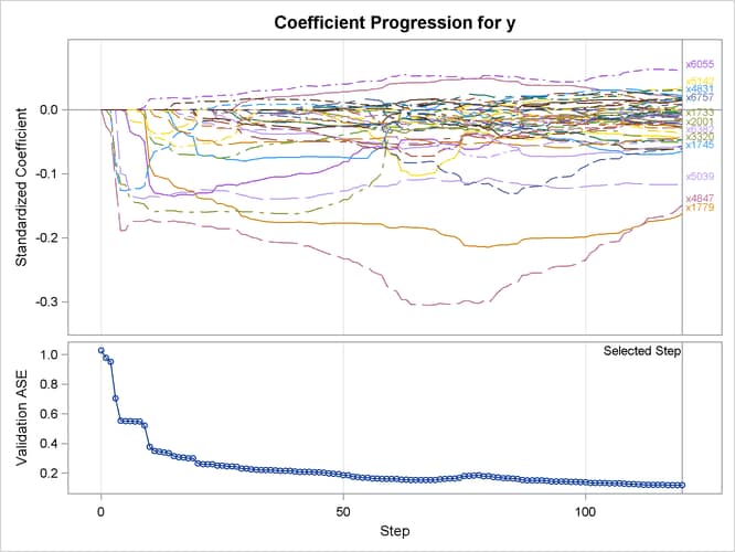
PROC GLMSELECT tries a series of candidate values for the ridge regression parameter, which you can control by using the L2HIGH=, L2LOW=, and L2SEARCH= options. The ridge regression parameter is set to the value that achieves the minimum validation ASE (see Figure 48.12 for an illustration). Output 48.6.7 shows the "Elastic Net Selection Summary" table. Compared to Output 48.6.5, where a ridge regression parameter is specified by the L2= option, this table shows that a slightly lower validation ASE is achieved as the value of the ridge regression parameter is optimized on the validation data set.
Output 48.6.7: Elastic Net Selection Summary Table
| The GLMSELECT Procedure |
| Elastic Net Selection Summary |
| Step | Effect Entered |
Effect Removed |
Number Effects In |
ASE | Validation ASE |
|---|---|---|---|---|---|
| 0 | Intercept | 1 | 0.8227 | 1.0287 | |
| 1 | x4847 | 2 | 0.7884 | 0.9787 | |
| 2 | x3320 | 3 | 0.7610 | 0.9508 | |
| 3 | x2020 | 4 | 0.4936 | 0.7061 | |
| 4 | x5039 | 5 | 0.2839 | 0.5527 | |
| 5 | x1249 | 6 | 0.2790 | 0.5519 | |
| 6 | x2242 | 7 | 0.2256 | 0.5513 | |
| . | . | . | |||
| . | . | . | |||
| . | . | . | |||
| 110 | x3605 | 49 | 0.0000 | 0.1252 | |
| 111 | x1975 | 50 | 0.0000 | 0.1241 | |
| 112 | x6757 | 51 | 0.0000 | 0.1224 | |
| 113 | x3221 | 50 | 0.0000 | 0.1206 | |
| 114 | x2183 | 51 | 0.0000 | 0.1205 | |
| 115 | x259 | 52 | 0.0000 | 0.1202 | |
| 116 | x157 | 53 | 0.0000 | 0.1201 | |
| 117 | x1781 | 54 | 0.0000 | 0.1197 | |
| 118 | x7065 | 53 | 0.0000 | 0.1194 | |
| 119 | x4079 | 54 | 0.0000 | 0.1187 | |
| 120 | x6539 | 55 | 0.0000 | 0.1186* | |
| * Optimal Value of Criterion | |||||
Output 48.6.8 shows the standardized coefficients of all the effects that are selected at some step of the elastic net method, plotted as a function of the step number.
When validation data are not available, you can use other criteria supported by the CHOOSE= option for estimating the value of the ridge regression parameter. Criteria such as AIC, AICC, and BIC are defined for the training samples only, and they tend to set the value of the ridge regression parameter to 0 when the number of training samples is less than the number of variables. In this case, the elastic net method reduces to the LASSO method. As an alternative to AIC, AICC, and BIC, you can use either k-fold cross validation or k-fold external cross validation in the CHOOSE= option, where the criterion is computed for held-out data.
If you want to use k-fold cross validation for selecting the model and selecting the appropriate value for the ridge regression parameter, you can use the following statements to apply the elastic net method of model selection:
proc glmselect data=sashelp.Leutrain testdata=sashelp.Leutest
               plots=coefficients;
   model y = x1-x7129/
         selection=elasticnet(steps=120 choose=cv)cvmethod=split(4);
run;
Output 48.6.9: Elastic Net Selection Summary Table
| The GLMSELECT Procedure |
| Elastic Net Selection Summary |
| Step | Effect Entered |
Effect Removed |
Number Effects In |
ASE | Test ASE | CV PRESS |
|---|---|---|---|---|---|---|
| 0 | Intercept | 1 | 0.8227 | 1.0287 | 31.4370 | |
| 1 | x4847 | 2 | 0.7884 | 0.9787 | 10.6957 | |
| 2 | x3320 | 3 | 0.7610 | 0.9507 | 10.2065 | |
| 3 | x2020 | 4 | 0.4935 | 0.7061 | 7.5478 | |
| 4 | x5039 | 5 | 0.2838 | 0.5527 | 5.7695 | |
| 5 | x1249 | 6 | 0.2790 | 0.5518 | 5.0187 | |
| 6 | x2242 | 7 | 0.2255 | 0.5513 | 5.4050 | |
| . | . | . | . | |||
| . | . | . | . | |||
| . | . | . | . | |||
| 80 | x4831 | 37 | 0.0000 | 0.1919 | 24.0303 | |
| 81 | x1745 | 38 | 0.0000 | 0.1933 | 24.0303 | |
| 82 | x4831 | 39 | 0.0000 | 0.1937 | 24.0303 | |
| 83 | x2661 | 40 | 0.0000 | 0.1864 | 24.0303 | |
| 84 | x3605 | 39 | 0.0000 | 0.1857 | 24.0303 | |
| 85 | x464 | 38 | 0.0000 | 0.1857 | 7.2724 | |
| 86 | x5766 | 39 | 0.0000 | 0.1854 | 7.2724 | |
| 87 | x464 | 40 | 0.0000 | 0.1763 | 7.2724 | |
| 88 | x6376 | 41 | 0.0000 | 0.1735 | 7.2724 | |
| 89 | x464 | 40 | 0.0000 | 0.1675 | 7.2724 | |
| 90 | x4079 | 39 | 0.0000 | 0.1674 | 1.2851 | |
| 91 | x1987 | 40 | 0.0000 | 0.1625 | 1.2846* | |
| * Optimal Value of Criterion | ||||||
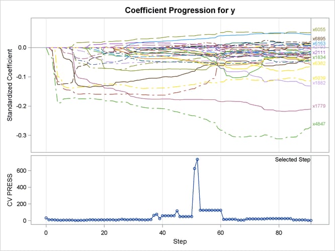
A TESTDATA= data set is named in the PROC GLMSELECT statement; this is the same as the validation data set used earlier. Because the L2= option is not specified, PROC GLMSELECT tries a series of candidate values for the ridge regression parameter according to the CHOOSE=CV option, and the ridge regression parameter is set to the value that achieves the minimal CVPRESS score. Output 48.6.9 shows the "Elastic Net Selection Summary" table, which corresponds to the ridge regression parameter selected by k-fold cross validation. The elastic net method achieves the smallest CVPRESS score at step 91. Hence the model at this step is selected, resulting in 40 selected effects.
Output 48.6.10 shows the standardized coefficients of all the effects selected at some step of the elastic net method, plotted as a function of the step number. Note that k-fold cross validation uses a least squares fit to compute the CVPRESS score. Thus the criterion does not directly depend on the penalized regression used in the elastic net method, and the CVPRESS curve in Output 48.6.10 has abrupt jumps.
If you want to perform the selection of both the ridge regression parameter and the selected variables in the model based on a criterion that directly depends on the regression used in the elastic net method, you can use k-fold external cross validation by specifying the following statements:
proc glmselect data=sashelp.Leutrain testdata=sashelp.Leutest
               plots=coefficients;
   model y = x1-x7129/
         selection=elasticnet(steps=120 choose=cvex)cvmethod=split(4);
run;
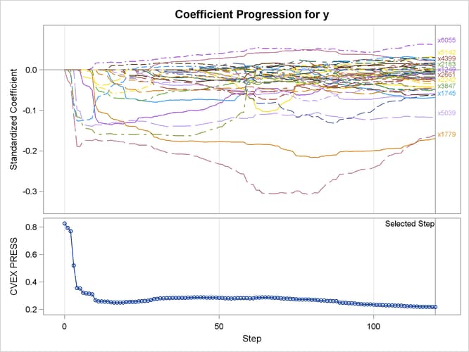
As earlier, a TESTDATA= data set is named in the PROC GLMSELECT statement to test the prediction accuracy of the model on the training samples. Because the L2= option is not specified, PROC GLMSELECT tries a series of candidate values for the ridge regression parameter. Output 48.6.11 shows the standardized coefficients of all the effects selected at some step of the elastic net method, plotted as a function of the step number, and also the curve of the CVEXPRESS statistic as a function of the step number. A comparison between the criterion curves in Output 48.6.10 and Output 48.6.11 shows that the CVEXPRESS statistic is smoother than the CVPRESS statistic. Note that the CVEXPRESS statistic is based on a penalized model, whereas the CVPRESS statistic is based on an ordinary least squares model. Output 48.6.12 shows the "Elastic Net Selection Summary" table, which corresponds to the ridge regression parameter selected by k-fold external cross validation. The elastic net method achieves the smallest CVEXPRESS score at step 120, and hence the model at this step is selected, resulting in 53 selected effects.
Output 48.6.12: Elastic Net Selection Summary Table
| The GLMSELECT Procedure |
| Elastic Net Selection Summary |
| Step | Effect Entered |
Effect Removed |
Number Effects In |
ASE | Test ASE | CVEX PRESS |
|---|---|---|---|---|---|---|
| 0 | Intercept | 1 | 0.8227 | 1.0287 | 0.8265 | |
| 1 | x4847 | 2 | 0.7884 | 0.9787 | 0.7940 | |
| 2 | x3320 | 3 | 0.7610 | 0.9507 | 0.7698 | |
| 3 | x2020 | 4 | 0.4936 | 0.7061 | 0.5195 | |
| 4 | x5039 | 5 | 0.2839 | 0.5527 | 0.3554 | |
| 5 | x1249 | 6 | 0.2790 | 0.5519 | 0.3526 | |
| 6 | x2242 | 7 | 0.2255 | 0.5513 | 0.3218 | |
| 7 | x6539 | 8 | 0.2161 | 0.5498 | 0.3166 | |
| 8 | x6055 | 9 | 0.2128 | 0.5488 | 0.3148 | |
| 9 | x1779 | 10 | 0.1968 | 0.5205 | 0.3096 | |
| 10 | x3847 | 11 | 0.1065 | 0.3765 | 0.2671 | |
| 11 | x4951 | 12 | 0.0891 | 0.3498 | 0.2586 | |
| 12 | x1834 | 13 | 0.0868 | 0.3458 | 0.2579 | |
| 13 | x1745 | 14 | 0.0837 | 0.3397 | 0.2570 | |
| 14 | x6021 | 15 | 0.0809 | 0.3355 | 0.2561 | |
| 15 | x6362 | 16 | 0.0667 | 0.3144 | 0.2510 | |
| 16 | x2238 | 17 | 0.0621 | 0.3075 | 0.2498 | |
| . | . | . | . | |||
| . | . | . | . | |||
| . | . | . | . | |||
| 100 | x2121 | 45 | 0.0000 | 0.1402 | 0.2350 | |
| 101 | x6021 | 46 | 0.0000 | 0.1386 | 0.2334 | |
| 102 | x3171 | 45 | 0.0000 | 0.1377 | 0.2324 | |
| 103 | x4461 | 46 | 0.0000 | 0.1350 | 0.2302 | |
| 104 | x4697 | 47 | 0.0000 | 0.1338 | 0.2299 | |
| 105 | x3605 | 46 | 0.0000 | 0.1331 | 0.2293 | |
| 106 | x3221 | 47 | 0.0000 | 0.1330 | 0.2289 | |
| 107 | x5002 | 48 | 0.0000 | 0.1320 | 0.2282 | |
| 108 | x3820 | 47 | 0.0000 | 0.1319 | 0.2281 | |
| 109 | x4697 | 46 | 0.0000 | 0.1315 | 0.2278 | |
| 110 | x4052 | 47 | 0.0000 | 0.1276 | 0.2235 | |
| 111 | x6184 | 48 | 0.0000 | 0.1266 | 0.2229 | |
| 112 | x3605 | 49 | 0.0000 | 0.1252 | 0.2215 | |
| 113 | x1975 | 50 | 0.0000 | 0.1240 | 0.2212 | |
| 114 | x6757 | 51 | 0.0000 | 0.1222 | 0.2200 | |
| 115 | x3221 | 50 | 0.0000 | 0.1206 | 0.2185 | |
| 116 | x2183 | 51 | 0.0000 | 0.1205 | 0.2185 | |
| 117 | x259 | 52 | 0.0000 | 0.1202 | 0.2182 | |
| 118 | x157 | 53 | 0.0000 | 0.1201 | 0.2181 | |
| 119 | x1781 | 54 | 0.0000 | 0.1197 | 0.2177 | |
| 120 | x7065 | 53 | 0.0000 | 0.1194 | 0.2177* | |
| * Optimal Value of Criterion | ||||||