The GLMSELECT Procedure
-
Overview

- Getting Started
-
Syntax
-
DetailsModel-Selection MethodsModel Selection IssuesCriteria Used in Model Selection MethodsCLASS Variable Parameterization and the SPLIT OptionMacro Variables Containing Selected ModelsUsing the STORE StatementBuilding the SSCP MatrixModel AveragingUsing Validation and Test DataCross ValidationExternal Cross ValidationScreeningDisplayed OutputODS Table NamesODS Graphics
-
Examples
- References
The method of cross validation that is discussed in the previous section judges models by their performance with respect to ordinary least squares. An alternative to ordinary least squares is to use the penalized regression that is defined by the LASSO or elastic net method. This method is called external cross validation, and you can specify external cross validation with CHOOSE=CVEX, new in SAS/STAT 13.1. CHOOSE=CVEX applies only when SELECTION=LASSO or SELECTION=ELASTICNET.
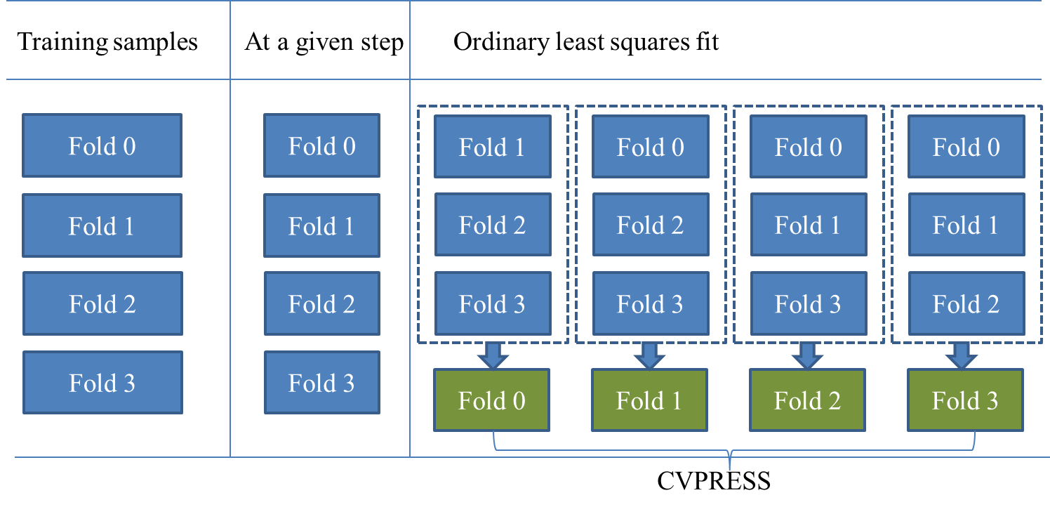
To understand how k-fold external cross validation works, first recall how k-fold cross validation works, as shown in Figure 48.18. The first column in this figure illustrates dividing the training samples into four folds, the second column illustrates the same training samples with reduced numbers of variables at a given step, and the third column illustrates applying ordinary least squares to compute the CVPRESS statistic. For the SELECTION=LASSO and SELECTION=ELASTICNET options, the CVPRESS statistic that is computed by k-fold cross validation uses an ordinary least squares fit, and hence it does not directly depend on the coefficients obtained by the penalized least squares regression.
If you want a statistic that is directly based on the coefficients obtained by a penalized least squares regression, you can specify CHOOSE=CVEX to use k-fold external cross validation. External cross validation directly applies the coefficients obtained by a penalized least squares regression to computing the predicted residual sum of squares. Figure 48.19 depicts k-fold external cross validation.
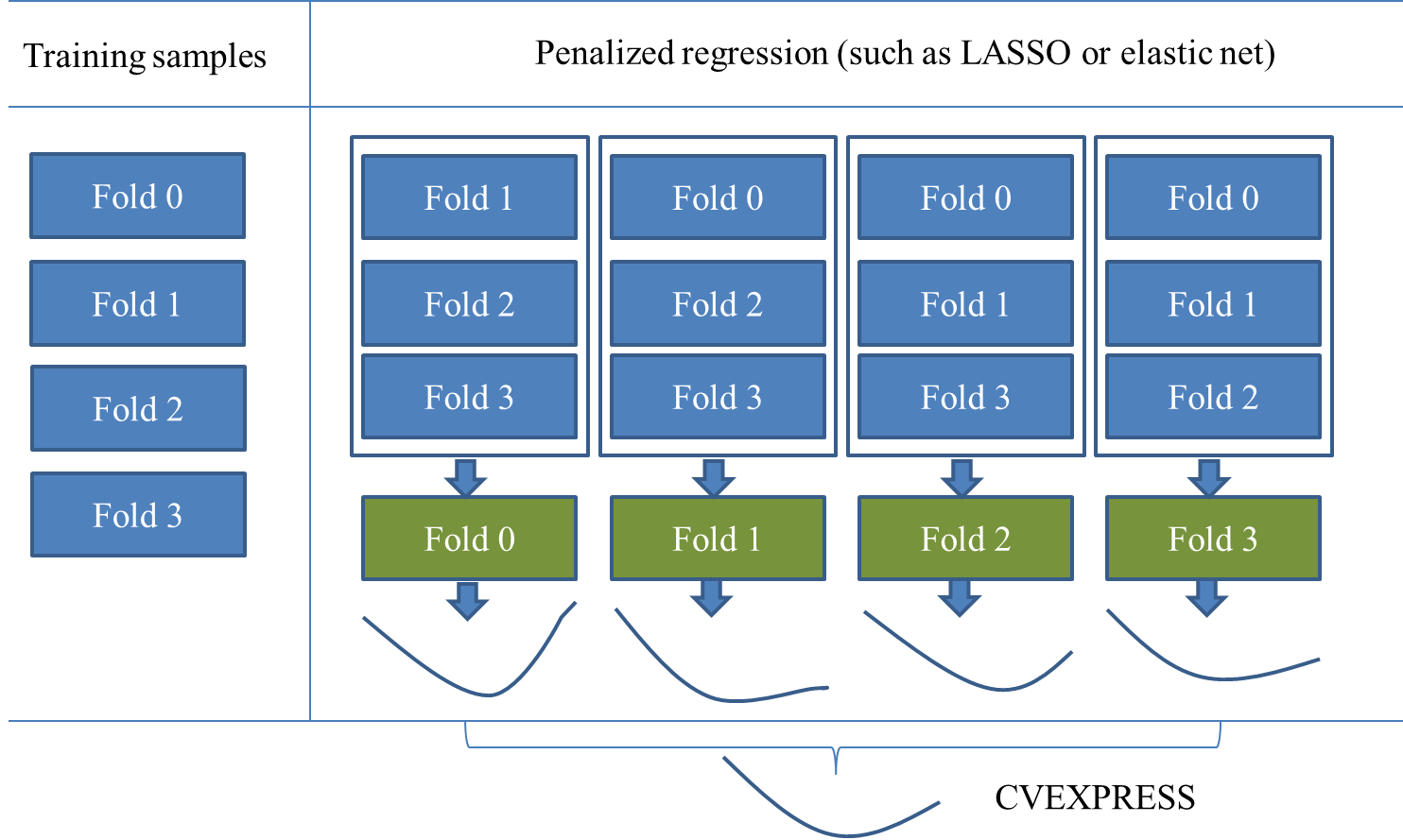
In k-fold external cross validation, the data are split into k approximately equal-sized parts, as illustrated in the first column of Figure 48.19. One of these parts is held out for validation, and the model is fit on the remaining ![]() parts by the LASSO method or the elastic net method. This fitted model is used to compute the predicted residual sum of squares
on the omitted part, and this process is repeated for each of the k parts. More specifically, for the ith model fit (
parts by the LASSO method or the elastic net method. This fitted model is used to compute the predicted residual sum of squares
on the omitted part, and this process is repeated for each of the k parts. More specifically, for the ith model fit (![]() ), let
), let ![]() denote the held-out part of the matrix of covariates and
denote the held-out part of the matrix of covariates and ![]() denote the corresponding response, and let
denote the corresponding response, and let ![]() denote the remaining
denote the remaining ![]() parts of the matrix of covariates and
parts of the matrix of covariates and ![]() denote the corresponding response. The LASSO method is applied on
denote the corresponding response. The LASSO method is applied on ![]() and
and ![]() to solve the optimization problem
to solve the optimization problem
Note that, as discussed in the section Elastic Net Selection (ELASTICNET), the elastic net method can be solved in the same way as LASSO, by augmenting the design matrix ![]() and the response
and the response ![]() .
.
Following the piecewise linear solution path of LASSO, the coefficients
are computed to correspond to the LASSO regularization parameter
Based on the computed coefficients, the predicted residual sum of squares is computed on the held-out part ![]() and
and ![]() as
as
The preceding process can be summarized as
For the illustration in Figure 48.19, the results ![]() correspond to four curves. The knots
correspond to four curves. The knots ![]() are usually different among different model fits
are usually different among different model fits ![]() . To merge the results of the k model fits for computing the CVEXPRESS statistic, perform the following three steps:
. To merge the results of the k model fits for computing the CVEXPRESS statistic, perform the following three steps:
- 1.
-
Identify distinct knots among all
- 2.
-
Apply interpolation to compute the predicted residual sum of squares at all the knots. Here the interpolation is done in a closed quadratic function by using the piecewise linear solutions of LASSO.
- 3.
-
Add the predicted residual sum of squares of k model fits according to the identified knots, and the sum of the k predicted residual sum of squares so obtained is the estimate of the prediction error that is denoted by CVEXPRESS.
The bottom curve in Figure 48.19 illustrates the curve between the CVEXPRESS statistics and the value of ![]() (L1). Note that computing the CVEXPRESS statistic for k-fold external cross validation requires fitting k different LASSO or elastic net models, and so the work and memory requirements increase linearly with the number of cross
validation folds.
(L1). Note that computing the CVEXPRESS statistic for k-fold external cross validation requires fitting k different LASSO or elastic net models, and so the work and memory requirements increase linearly with the number of cross
validation folds.
In addition to characterizing the piecewise linear solutions of the coefficients ![]() by the LASSO regularization parameters
by the LASSO regularization parameters ![]() , you can also characterize the solutions by the sum of the absolute values of the coefficients or the scaled regularization
parameter. For a detailed discussion of the different options, see the L1CHOICE=
option in the MODEL
statement.
, you can also characterize the solutions by the sum of the absolute values of the coefficients or the scaled regularization
parameter. For a detailed discussion of the different options, see the L1CHOICE=
option in the MODEL
statement.
Like k-fold cross validation, you can use the CVMETHOD=
option in the MODEL
statement to specify the method for splitting the data into k parts in k-fold external cross validation. CVMETHOD=
BLOCK(k) requests that the k parts be made of blocks of ![]() or
or ![]() successive observations, where n is the number of observations. CVMETHOD=
SPLIT(k) requests that parts consist of observations
successive observations, where n is the number of observations. CVMETHOD=
SPLIT(k) requests that parts consist of observations ![]() ,
, ![]() , . . . ,
, . . . , ![]() . CVMETHOD=
RANDOM(k) partitions the data into random subsets, each with approximately
. CVMETHOD=
RANDOM(k) partitions the data into random subsets, each with approximately ![]() observations. Finally, you can use the formatted value of an input data set variable to define the parts by specifying CVMETHOD=variable
. This last partitioning method is useful in cases where you need to exercise extra control over how the data are partitioned
by taking into account factors such as important but rare observations that you want to "spread out" across the various parts.
By default, PROC GLMSELECT uses CVMETHOD=
RANDOM(5) for external cross validation.
observations. Finally, you can use the formatted value of an input data set variable to define the parts by specifying CVMETHOD=variable
. This last partitioning method is useful in cases where you need to exercise extra control over how the data are partitioned
by taking into account factors such as important but rare observations that you want to "spread out" across the various parts.
By default, PROC GLMSELECT uses CVMETHOD=
RANDOM(5) for external cross validation.
For the elastic net method, if the ridge regression parameter ![]() is not specified by the L2= option and you use k-fold external cross validation for the CHOOSE= option, then the optimal
is not specified by the L2= option and you use k-fold external cross validation for the CHOOSE= option, then the optimal ![]() is searched over an interval (see Figure 48.12 for an illustration) and it is set to the value that achieves the minimum CVEXPRESS statistic. You can use the L2SEARCH=,
L2LOW=, L2HIGH=, and L2STEPS= options to control the search of
is searched over an interval (see Figure 48.12 for an illustration) and it is set to the value that achieves the minimum CVEXPRESS statistic. You can use the L2SEARCH=,
L2LOW=, L2HIGH=, and L2STEPS= options to control the search of ![]() (L2).
(L2).
If you specify SELECTION=LASSO or SELECTION=ELASTICNET, the penalized model is fit only once using the same training samples in k-fold cross validation, whereas the penalized model is fit k times by using different training samples in k-fold external cross validation. External cross validation also requires identifying the knots that result from the different solution paths. The CVPRESS statistic that is computed in k-fold cross validation is based on ordinary least squares regression, whereas the CVEXPRESS statistic that is computed in k-fold external cross validation is based on the penalized regression.
When you specify the CHOOSE= CVEX suboption of the SELECTION= option in the MODEL statement, the CVEXPRESS statistics are computed for the models at each step of the selection process. The model at the first step that has the smallest CVEXPRESS score is selected.