The GEE Procedure (Experimental)

Example 42.3 Weighted GEE for Longitudinal Data That Have Missing Values

This example shows how you can use the GEE procedure to analyze longitudinal data that contain missing values. The data set is taken from a longitudinal study of women who used contraception during four consecutive months (Fitzmaurice, Laird, and Ware, 2011). In this study, 1,151 women were randomly assigned to one of two treatments: 100 mg or 150 mg of depot-medroxyprogesterone acetate (DPMA). The response variable indicates their amenorrhea status in each of the four months. The question of interest is whether the treatment has an effect on the rate of the amenorrhea over time. The example follows the analysis done by Fitzmaurice, Laird, and Ware (2011).

The following statements create the data set Amenorrhea:

data Amenorrhea;
   input ID Dose Time Y@@;
   datalines;
   1     0       1     0
   1     0       2     .
   1     0       3     .
   1     0       4     .

   ... more lines ...   

1150     1       4     1
1151     1       1     1
1151     1       2     1
1151     1       3     1
1151     1       4     1
;

The variables in the data are as follows:

ID: patient’s ID
Y: indicator of amenorrhea status (1 for amenorrhea; 0 otherwise)
Time: four consecutive months with values 0, 1, 2, and 3
Dose: 0 for treatment with 100 mg injection; 1 for treatment with 150 mg injection

To prepare for the analysis, two additional variables are created:

Prevy: the patient’s amenorrhea status in the previous month. For the first month, this is set to an arbitrary nonmissing value (0 here). In this release of PROC GEE, this arbitrary value must be nonmissing and valid for the response variable—for example, it should be 0 or 1 for a binary response—but it does not otherwise affect the results.
Ctime: a copy of Time, which you can include in the marginal model as a continuous effect and also in the missingness model as a classification effect

The following statements add these two variables to the data set:

data Amenorrhea;
   set Amenorrhea;
   by ID;
   Prevy=lag(Y);
   if first.id then Prevy=0;
   Time=Time-1;
   Ctime=Time;
run;

Suppose $y_{ij}$ denotes the amenorrhea status of woman i at the jth visit, $j=1,\ldots ,4$ , and suppose $\mu _{ij}=\mr{P}(y_{ij}=1)$ denotes the average rate of high dosage. To explore whether the treatment has an effect on the rate of amenorrhea over time, consider the following marginal model:

$\mr{logit}(\mu _{ij}) = \beta _0 + \beta _1 \mr{time}_{ij} + \beta _2 \mr{time}_{ij}^2+ \beta _3 \mr{dose}_ i + \beta _4 \mr{dose}_ i \times \mr{time} + \beta _5 \mr{dose}_ i \times \mr{time}^2$

Of the 1,151 women in this study, 576 are from the low-dose group, and 575 are from the high-dose group. For the low-dose group, 62.67% of the women completed the trial; for the high-dose group, 61.39% of the women completed this trial. Thus, both groups have substantial dropouts.

To obtain the weights for the weighted GEE analysis, consider the following logistic regression model for missingness:

$\begin{align*} \mr{logit}p(r_{ij}=1|r_{ij-1}=1,\mr{dose}_{i},\mr{time}_{ij},y_{ij-1})=& \alpha _0 + \alpha _1 I(\mr{time}_{ij}=2) + \alpha _2 I(\mr{time}_{ij}=3) \\ & +\alpha _3 \mr{dose}_ i + \alpha _4 y_{ij-1}+ \alpha _5 \mr{dose}_ i \times y_{ij-1} \end{align*}$

The following statements use the observation-specific weighted GEE method and the specified response and missingness models to analyze the data:

ods graphics on;
proc gee data=Amenorrhea desc plots=histogram;
   class ID Ctime;
   missmodel Ctime Prevy Dose Dose*Prevy / type=obslevel;
   model Y = Time Dose Time*Time Dose*Time Dose*Time*Time / dist=bin;
   repeated subject=ID / within=Ctime corr=cs;
run;

The MODEL statement specifies logistic regression and the model effects. The DESCEND option in the PROC GEE statement models the probability that Y = 1.

The REPEATED statement requests GEE analysis. The SUBJECT=ID option specifies that observations from the same subject are identified by ID. The TYPE=CS option specifies the compound symmetric working correlation structure.

The MISSMODEL statement requests the weighted GEE analysis. It specifies the logistic regression model for missingness. Note that no response variable is needed in weighted GEE analysis to specify a missingness model because the response is completely determined by the response variable in the MODEL statement. Without the MISSMODEL statement, PROC GEE would use the standard GEE approach, the same as provided by PROC GENMOD. The TYPE=OBSLEVEL option requests observation-specific weights.

Output 42.3.1 shows the parameter estimates for the missingness model. The estimate of $\alpha _4$ is –0.4514 with a p-value of 0.0053, which suggests that the possibility that a participant will drop out is related to her previous amenorrhea status. This suggests that the assumption of MAR is more appropriate than that of MCAR.

Output 42.3.1: Parameter Estimates for the Missingness Model

Parameter Estimates for Missingness Model
Parameter		Estimate	Standard Error	95% Confidence Limits		Z	Pr > \|Z\|
Intercept		2.3967	0.1438	2.1149	2.6785	16.67	<.0001
Ctime	0	0.0000	0.0000	0.0000	0.0000	.	.
Ctime	1	-0.7286	0.1439	-1.0106	-0.4466	-5.06	<.0001
Ctime	2	-0.5919	0.1469	-0.8798	-0.3040	-4.03	<.0001
Ctime	3	0.0000	0.0000	0.0000	0.0000	.	.
Prevy		-0.4514	0.1619	-0.7687	-0.1341	-2.79	0.0053
Dose		0.0680	0.1313	-0.1893	0.3253	0.52	0.6046
Prevy*Dose		-0.2381	0.2196	-0.6685	0.1923	-1.08	0.2782

Output 42.3.2 displays the results of the weighted GEE analysis.

Output 42.3.2: Parameter Estimates for Amenorrhea Data Analysis Using Weighted GEE

The GEE Procedure

Parameter Estimates for Response Model
with Empirical Standard Error
Parameter	Estimate	Standard Error	95% Confidence Limits		Z	Pr > \|Z\|
Intercept	-1.4965	0.1072	-1.7067	-1.2863	-13.95	<.0001
Time	0.5379	0.1334	0.2764	0.7994	4.03	<.0001
Dose	0.1061	0.1491	-0.1861	0.3983	0.71	0.4767
Time*Time	-0.0037	0.0405	-0.0831	0.0757	-0.09	0.9275
Dose*Time	0.4092	0.1903	0.0362	0.7823	2.15	0.0315
DoseTimeTime	-0.1264	0.0577	-0.2395	-0.0134	-2.19	0.0284

The estimate of $\beta _4$ (the parameter estimate for the Dose*Time interaction) is 0.4092, which indicates that the change of amenorrhea rate over time depends on the dose of DMPA. Specifically, for women in the low-dose group, the amenorrhea rates $\mu _{ij}$ at the four consecutive time intervals are 0.1830, 0.2764, 0.3928, and 0.5210 and for women in the high-dose group, the amenorrhea rate are 0.1997, 0.3609, 0.4963, and 0.5701. In other words, the amenorrhea rate increases over time for both treatments, and the rates of increase are slightly different.

You can request subject-level weights by specifying the TYPE=SUBLEVEL option. The results (not shown here) from the subject-level weighted method are similar to the results from the observation-level weighted method. Both of the weighted GEE methods provide unbiased regression parameter estimates if the missingness model is specified correctly. Preisser, Lohman, and Rathouz (2002) note that the observation-level weighted GEE produces more efficient estimates than the cluster-level weighted GEE produces for incomplete longitudinal binary data.

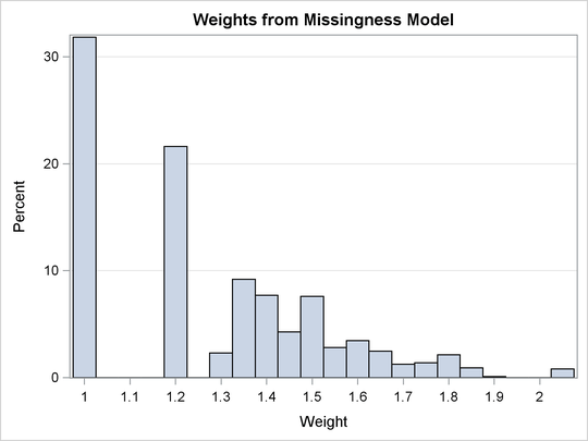
Large weights can have impacts on the parameter estimates. Consequently, it is recommended that you check the distribution of the estimated weights. If there are large weights, you might consider trimming them by specifying the MAXWEIGHT= option in the MISSMODEL statement. Output 42.3.3 shows that the estimated weights in this example range between 1 and 2.1, so no trimming is needed.

Output 42.3.3: Histogram of Estimated Weights