The BCHOICE Procedure

The BCHOICE (Bayesian choice) procedure performs Bayesian analysis for discrete choice models. Discrete choice models are used in marketing research to model decision makers’ choices among alternative products and services. The decision maker might be people, households, companies and so on, and the alternatives might be products, services, actions, or any other options or items about which choices must be made (Train, 2009). The collection of alternatives that are available to the decision makers is called a choice set.
Discrete choice models are derived under the assumption of utility-maximizing behavior by decision makers. When individuals are asked to make one choice among a set of alternatives, they usually determine the level of utility that each alternative offers. The utility that individual i obtains from alternative j among J alternatives is denoted as
where the subscript i is an index for the individuals, the subscript j is an index for the alternatives in a choice set, ![]() is a nonstochastic utility function that relates observed factors to the utility, and
is a nonstochastic utility function that relates observed factors to the utility, and ![]() is the error component that captures the unobserved characteristics of the utility. In discrete choice models, the observed
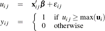
part of the utility function is assumed to be linear in the parameters,
is the error component that captures the unobserved characteristics of the utility. In discrete choice models, the observed
part of the utility function is assumed to be linear in the parameters,
where ![]() is a p-dimensional design vector of observed attribute levels that relate to alternative j and
is a p-dimensional design vector of observed attribute levels that relate to alternative j and ![]() is the corresponding vector of fixed regression coefficients that indicate the utilities or part-worths of the attribute
levels.
is the corresponding vector of fixed regression coefficients that indicate the utilities or part-worths of the attribute
levels.
Decision makers choose the alternative that gives them the greatest utility. Let ![]() be the multinomial response vector for the ith individual. The value
be the multinomial response vector for the ith individual. The value ![]() takes 1 if the jth component of
takes 1 if the jth component of ![]() is the largest, and 0 otherwise:
is the largest, and 0 otherwise:
Different specifications about the density of the error vector ![]() result in different types of choice models: logit, nested logit, and probit, as detailed in the section Types of Choice Models. Logit and nested logit models have closed-form likelihood, whereas a probit model does not.
result in different types of choice models: logit, nested logit, and probit, as detailed in the section Types of Choice Models. Logit and nested logit models have closed-form likelihood, whereas a probit model does not.
The past 15 years have seen a dramatic increase in using a Bayesian approach to develop new methods of analysis and models of consumer behavior. The milestone breakthroughs are Albert and Chib (1993) and McCulloch and Rossi (1994) for choice probit models, and Allenby and Lenk (1994) and Allenby (1997) for logit models that have normally distributed random effects (these models are called mixed logit models). Train (2009) extends the Bayesian procedure for mixed logit models to include nonnormal distributions, such as lognormal, uniform, and triangular distributions.
An issue in choice models is that the quantity of relevant data at the individual level is very limited. Respondents frequently become fatigued after answering 15 to 20 questions in a survey. Rossi, McCulloch, and Allenby (1996) and Allenby and Rossi (1999) show how to obtain information about individual-level parameters within a model by using random taste variation. The lack of data at the individual level, combined with the desire to account for individual differences instead of treating all respondents alike, presents challenges in marketing research. Bayesian methods are ideally suited for analyzing limited data.
Bayesian methods have several advantages. First, Bayesian methods do not require optimization of any function. For probit models and logit models that have random effects, optimization of the likelihood function can be numerically difficult. Different starting values might lead to different maximization results. The problem of a local maximum versus a global maximum is another issue, because convergence is not guaranteed to find the global maximum. Second, Bayesian procedures enable consistency and efficiency to be achieved under more relaxed conditions. When the likelihood function does not have a closed form or there are too many parameters (as in models with random effects), simulation can be used to estimate the likelihood function. Maximization that is based on such a simulated likelihood function is consistent only if the number of draws in simulation rises with the sample size, and it is efficient only if the number of draws in simulation increases faster than the square root of the sample size. On the other hand, Bayesian methods are consistent for a fixed number of draws and are efficient if the number of draws goes up at any rate with the sample size.
For a short introduction to Bayesian analysis and related basic concepts, see Chapter 7: Introduction to Bayesian Analysis Procedures. Also see the section A Bayesian Reading List for a guide to Bayesian textbooks of varying degrees of difficulty. It follows from Bayes’ theorem that a posterior distribution is proportional to the product of the likelihood function and the prior distribution of the parameter. When it is difficult to obtain the posterior distribution analytically, Bayesian methods often rely on simulations to generate samples from the posterior distribution, and they use the simulated draws to approximate the distribution and to make the inferences.
To use the BCHOICE procedure, you need to specify the type of model for the data. You can also supply a prior distribution for the parameters if you want something other than the default noninformative prior. PROC BCHOICE obtains samples from the corresponding posterior distributions, produces summary and diagnostic statistics, and saves the posterior samples in an output data set that can be used for further analysis. The procedure derives inferences from simulation rather than through analytic or numerical methods. You should expect slightly different answers from each run for the same problem, unless you use the same random number seed.