The BCHOICE Procedure

Choice models that have random effects (or random coefficients) provide solutions to create individual-level or group-specific utilities. They are also referred as "mixed models" or "hybrid models." One of the greatest challenges in marketing research is to account for the diversity of preferences and sensitivities in the marketplace. Heterogeneity in individual preferences is the reason for differentiated product programs and market segmentation. As individual preferences become more diverse, it becomes less appropriate to consider the analyses in an aggregated way. Individual utilities are useful because they make segmentation easy and provide a way to detect groups. Because people have different preferences, it can be misleading to roll the whole sample together into a single set of utilities.
For example, imagine studying the popularity of a new brand. Some participants in the study who are interviewed love the new brand, whereas others dislike it. If you simply aggregate the data and look at the average, the conclusion is that the sample is ambivalent toward the new brand. This would be the least helpful conclusion that could be drawn, because it does not fit for anyone.
Choice models that have random effects generalize the standard choice models to incorporate individual-level effects. Let
the utility that individual i obtains from alternative j in choice situation t (![]() ) be
) be
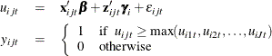
where ![]() is the observed choice for individual i and alternative j in choice situation t;
is the observed choice for individual i and alternative j in choice situation t; ![]() is the fixed design vector for individual i and alternative j in choice situation t;
is the fixed design vector for individual i and alternative j in choice situation t; ![]() is the vector of fixed coefficients;
is the vector of fixed coefficients; ![]() is the random design vector for individual i and alternative j in choice situation t; and
is the random design vector for individual i and alternative j in choice situation t; and ![]() is the vector of random coefficients for individual i that correspond to
is the vector of random coefficients for individual i that correspond to ![]() . Sometimes the random coefficients might be at a level different from the individual level. For example, it is common to
assume that there are random coefficients at the household level or group level of participants. For the convenience of notation,
random effects are assumed to be at the individual level.
. Sometimes the random coefficients might be at a level different from the individual level. For example, it is common to
assume that there are random coefficients at the household level or group level of participants. For the convenience of notation,
random effects are assumed to be at the individual level.
In the random-effects model, it is assumed that each ![]() is drawn from a superpopulation and this superpopulation is normal,
is drawn from a superpopulation and this superpopulation is normal, ![]() . An additional stage is added to the model where a prior for
. An additional stage is added to the model where a prior for ![]() is specified:
is specified:
The covariance matrix ![]() characterizes the extent of heterogeneity among individuals. Large diagonal elements of
characterizes the extent of heterogeneity among individuals. Large diagonal elements of ![]() indicate substantial heterogeneity in part-worths. Off-diagonal elements indicate patterns in the evaluation of attribute
levels. For example, positive covariances specify pairs of attribute levels that tend to be evaluated similarly across respondents.
Product offerings that consist of these attribute levels are more strongly preferred or disliked by certain individuals.
indicate substantial heterogeneity in part-worths. Off-diagonal elements indicate patterns in the evaluation of attribute
levels. For example, positive covariances specify pairs of attribute levels that tend to be evaluated similarly across respondents.
Product offerings that consist of these attribute levels are more strongly preferred or disliked by certain individuals.
In this setup, the prior mean is 0 for the random effects, meaning that the random effects either are truly around 0 or have
been centered by the fixed effects. For random effects whose mean is not around 0, you can follow the usual practice of specifying
them in the fixed effects. For example, if one random effect is price and you do not think that the population mean of price is around 0, then you should add price as a fixed effect as follows:
proc bchoice data=randeffdata;
   class subj set;
   model y = price / choiceset=(subj set);
   random  price / subject=subj;
run;
Thus, you obtain the estimate for the population mean of the price effect through the fixed effect, and you obtain the deviation from the population mean for each individual through random
effects.
Allenby and Rossi (1999) and Rossi, Allenby, and McCulloch (2005) propose a hierarchical Bayesian random-effects model that is set up in a different way. In their model, there are no fixed effects but only random effects. This model, which is referred to as the random-effects-only model in the rest of this chapter, is as follows:
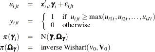
where ![]() is a mean vector of regression coefficients, which models the central location of distribution of the random coefficients;
is a mean vector of regression coefficients, which models the central location of distribution of the random coefficients;
![]() represents the average part-worths across the respondents in the data. If you want to use this setup, specify the REMEAN
option in the RANDOM
statement to request estimation on
represents the average part-worths across the respondents in the data. If you want to use this setup, specify the REMEAN
option in the RANDOM
statement to request estimation on ![]() and do not specify any fixed effects in the MODEL
statement.
and do not specify any fixed effects in the MODEL
statement.
Rossi, McCulloch, and Allenby (1996) and Rossi, Allenby, and McCulloch (2005) add another layer of flexibility to the random-effects-only model by allowing heterogeneity that is driven by observable (demographic) characteristics of the individuals. They model the prior mean of the random coefficients as a function of the individual’s demographic variables (such as age and gender),
where ![]() is a vector that consists of an intercept and some observable demographic variables.
is a vector that consists of an intercept and some observable demographic variables. ![]() is a matrix of regression coefficients, which affects the location of distribution of the random coefficients.
is a matrix of regression coefficients, which affects the location of distribution of the random coefficients. ![]() should be useful for identifying respondents who have part-worths that are different from those in the rest of the sample
if some individual-level characteristics are included in
should be useful for identifying respondents who have part-worths that are different from those in the rest of the sample
if some individual-level characteristics are included in ![]() . This specification allows the preferences or intercepts to vary by both demographic variables and the slopes. If
. This specification allows the preferences or intercepts to vary by both demographic variables and the slopes. If ![]() consists of only an intercept, this model reduces to the previous one. For more information about how to sample
consists of only an intercept, this model reduces to the previous one. For more information about how to sample ![]() , see Rossi, McCulloch, and Allenby (1996), Rossi, Allenby, and McCulloch (2005) (Section 2.12 in Chapter 2), and Rossi (2012).
, see Rossi, McCulloch, and Allenby (1996), Rossi, Allenby, and McCulloch (2005) (Section 2.12 in Chapter 2), and Rossi (2012).
The logit model with random effects consists of the fixed-coefficients parameters ![]() , the random-coefficients parameters
, the random-coefficients parameters ![]() , and the covariance parameters for the random coefficients
, and the covariance parameters for the random coefficients ![]() . You can use the Metropolis-Hastings sampling with Gamerman approach to draw samples through the following three conditional
posterior distributions:
. You can use the Metropolis-Hastings sampling with Gamerman approach to draw samples through the following three conditional
posterior distributions:
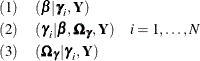
All chains are initialized with random effects that are set to 0 and a covariance matrix that is set to an identity matrix.
Updating is done first for the fixed effects, ![]() , as a block to position the chain in the correct region of the parameter space. Then the random effects are updated, and
finally the covariance of the random effects is updated. For more information, see Gamerman (1997) and the section Gamerman Algorithm.
, as a block to position the chain in the correct region of the parameter space. Then the random effects are updated, and
finally the covariance of the random effects is updated. For more information, see Gamerman (1997) and the section Gamerman Algorithm.
The hierarchical Bayesian random-effects-only model as proposed in Allenby and Rossi (1999) and Rossi, Allenby, and McCulloch (2005) contains the random-coefficients parameters ![]() , the population mean of the random-coefficients parameters
, the population mean of the random-coefficients parameters ![]() , and the covariance parameters for the random coefficients
, and the covariance parameters for the random coefficients ![]() . The sampling can be carried out by the following conditional posteriors:
. The sampling can be carried out by the following conditional posteriors:
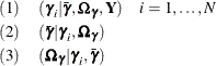
The second and third conditional posteriors are easy to draw because they have direct sampling distributions: the second
has a normal distribution with a mean of ![]() and a covariance of
and a covariance of ![]() ; the third is an
; the third is an ![]() , where
, where ![]() . There is no closed form for the first conditional posterior. The Metropolis-Hastings sampling with Gamerman approach is
the default sampling algorithm for it.
. There is no closed form for the first conditional posterior. The Metropolis-Hastings sampling with Gamerman approach is
the default sampling algorithm for it.
You can also use random walk Metropolis sampling when direct sampling is not an option, such as for the fixed-coefficients
parameters ![]() and random-coefficients parameters
and random-coefficients parameters ![]() . You can specify ALGORITHM
=RWM to choose random walk Metropolis sampling. For the random-coefficients parameters
. You can specify ALGORITHM
=RWM to choose random walk Metropolis sampling. For the random-coefficients parameters ![]() , Rossi, McCulloch, and Allenby (1996) and Rossi, Allenby, and McCulloch (2005) suggest random walk Metropolis sampling in which increments have covariance
, Rossi, McCulloch, and Allenby (1996) and Rossi, Allenby, and McCulloch (2005) suggest random walk Metropolis sampling in which increments have covariance ![]() , where s is a scaling constant whose value is usually set at
, where s is a scaling constant whose value is usually set at ![]() and
and ![]() is the current draw of
is the current draw of ![]() .
.
The sampling for the random-effects-only setup is often faster, because the first conditional posterior for each i involves only the data for individual i and because the second and third conditional posteriors depend not on the data directly but only on the draws of ![]() .
.
The probit model with random effects has the following parameters: the fixed-coefficients parameters ![]() , the covariance parameters for the error differences
, the covariance parameters for the error differences ![]() , the random-coefficients parameters
, the random-coefficients parameters ![]() , and the covariance parameters for the random coefficients
, and the covariance parameters for the random coefficients ![]() . It has extra parameters
. It has extra parameters ![]() in addition to
in addition to ![]() in a fixed-effects-only model. You can conveniently adapt the Gibbs sampler proposed in McCulloch and Rossi (1994) to handle the model by appending the new parameters to the set of parameters that would be drawn for a probit model without
random coefficients. The sampling can be carried out by the following conditional posteriors:
in a fixed-effects-only model. You can conveniently adapt the Gibbs sampler proposed in McCulloch and Rossi (1994) to handle the model by appending the new parameters to the set of parameters that would be drawn for a probit model without
random coefficients. The sampling can be carried out by the following conditional posteriors:
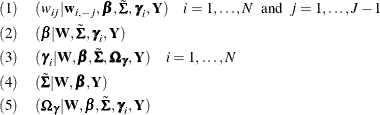
All the groups of conditional distributions have closed forms that are easily drawn from. Conditional (1) is truncated normal, (2) and (3) are normal, and (4) and (5) are inverse Wishart distribution. For more information, see McCulloch and Rossi (1994).