The LOGISTIC Procedure
- Overview
- Getting Started
-
Syntax
 PROC LOGISTIC StatementBY StatementCLASS StatementCODE StatementCONTRAST StatementEFFECT StatementEFFECTPLOT StatementESTIMATE StatementEXACT StatementEXACTOPTIONS StatementFREQ StatementID StatementLSMEANS StatementLSMESTIMATE StatementMODEL StatementNLOPTIONS StatementODDSRATIO StatementOUTPUT StatementROC StatementROCCONTRAST StatementSCORE StatementSLICE StatementSTORE StatementSTRATA StatementTEST StatementUNITS StatementWEIGHT Statement
 -
DetailsMissing ValuesResponse Level OrderingLink Functions and the Corresponding DistributionsDetermining Observations for Likelihood ContributionsIterative Algorithms for Model FittingConvergence CriteriaExistence of Maximum Likelihood EstimatesEffect-Selection MethodsModel Fitting InformationGeneralized Coefficient of DeterminationScore Statistics and TestsConfidence Intervals for ParametersOdds Ratio EstimationRank Correlation of Observed Responses and Predicted ProbabilitiesLinear Predictor, Predicted Probability, and Confidence LimitsClassification TableOverdispersionThe Hosmer-Lemeshow Goodness-of-Fit TestReceiver Operating Characteristic CurvesTesting Linear Hypotheses about the Regression CoefficientsRegression DiagnosticsScoring Data SetsConditional Logistic RegressionExact Conditional Logistic RegressionInput and Output Data SetsComputational ResourcesDisplayed OutputODS Table NamesODS Graphics
-
ExamplesStepwise Logistic Regression and Predicted ValuesLogistic Modeling with Categorical PredictorsOrdinal Logistic RegressionNominal Response Data: Generalized Logits ModelStratified SamplingLogistic Regression DiagnosticsROC Curve, Customized Odds Ratios, Goodness-of-Fit Statistics, R-Square, and Confidence LimitsComparing Receiver Operating Characteristic CurvesGoodness-of-Fit Tests and SubpopulationsOverdispersionConditional Logistic Regression for Matched Pairs DataFirth’s Penalized Likelihood Compared with Other ApproachesComplementary Log-Log Model for Infection RatesComplementary Log-Log Model for Interval-Censored Survival TimesScoring Data SetsUsing the LSMEANS StatementPartial Proportional Odds Model
- References
The memory needed to fit an unconditional model is approximately ![]() bytes, where p is the number of parameters estimated and n is the number of observations in the data set. For cumulative response models with more than two response levels, a test
of the parallel lines assumption requires an additional memory of approximately
bytes, where p is the number of parameters estimated and n is the number of observations in the data set. For cumulative response models with more than two response levels, a test
of the parallel lines assumption requires an additional memory of approximately ![]() bytes, where k is the number of response levels and m is the number of slope parameters. However, if this additional memory is not available, the procedure skips the test and
finishes the other computations. You might need more memory if you use the SELECTION= option for model building.
bytes, where k is the number of response levels and m is the number of slope parameters. However, if this additional memory is not available, the procedure skips the test and
finishes the other computations. You might need more memory if you use the SELECTION= option for model building.
The data that consist of relevant variables (including the design variables for model effects) and observations for fitting
the model are stored in a temporary utility file. If sufficient memory is available, such data will also be kept in memory;
otherwise, the data are reread from the utility file for each evaluation of the likelihood function and its derivatives, with
the resulting execution time of the procedure substantially increased. Specifying the MULTIPASS option in the MODEL statement avoids creating this utility file and also does not store the data in memory; instead, the DATA= data set is reread
when needed. This saves approximately ![]() bytes of memory but increases the execution time.
bytes of memory but increases the execution time.
If a conditional logistic regression is performed, then approximately ![]() additional bytes of memory are needed, where
additional bytes of memory are needed, where ![]() is the number of events in stratum h, H is the total number of strata, and
is the number of events in stratum h, H is the total number of strata, and ![]() is the number of variables used to define the strata. If the CHECKDEPENDENCY=ALL option is specified in the STRATA statement, then an extra
is the number of variables used to define the strata. If the CHECKDEPENDENCY=ALL option is specified in the STRATA statement, then an extra ![]() bytes are required, and the resulting execution time of the procedure might be substantially increased.
bytes are required, and the resulting execution time of the procedure might be substantially increased.
Many problems require a prohibitive amount of time and memory for exact computations, depending on the speed and memory available on your computer. For such problems, consider whether exact methods are really necessary. Stokes, Davis, and Koch (2012) suggest looking at exact p-values when the sample size is small and the approximate p-values from the unconditional analysis are less than 0.10, and they provide rules of thumb for determining when various models are valid.
A formula does not exist that can predict the amount of time and memory necessary to generate the exact conditional distributions
for a particular problem. The time and memory required depends on several factors, including the total sample size, the number
of parameters of interest, the number of nuisance parameters, and the order in which the parameters are processed. To provide
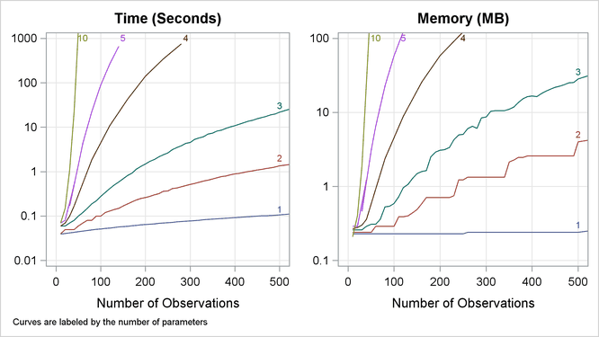
a feel for how these factors affect performance, 19 data sets containing Nobs ![]() observations consisting of up to 10 independent uniform binary covariates (
observations consisting of up to 10 independent uniform binary covariates (X1,…,XN) and a binary response variable (Y), are generated, and the following statements create exact conditional distributions for X1 conditional on the other covariates by using the default METHOD=NETWORK. Figure 58.11 displays results obtained on a 400Mhz PC with 768MB RAM running Microsoft Windows NT.
data one;
do obs=1 to HalfNobsXN…XN…XN
At any time while PROC LOGISTIC is deriving the distributions, you can terminate the computations by pressing the system interrupt key sequence (see the SAS Companion for your system) and choosing to stop computations. If you run out of memory, see the SAS Companion for your system to see how to allocate more.
You can use the EXACTOPTIONS option MAXTIME= to limit the total amount of time PROC LOGISTIC uses to derive all of the exact distributions. If PROC LOGISTIC does not finish within that time, the procedure terminates.
Calculation of frequencies are performed in the log scale by default. This reduces the need to check for excessively large frequencies but can be slower than not scaling. You can turn off the log scaling by specifying the NOLOGSCALE option in the EXACTOPTIONS statement. If a frequency in the exact distribution is larger than the largest integer that can be held in double precision, a warning is printed to the SAS log. But since inaccuracies due to adding small numbers to these large frequencies might have little or no effect on the statistics, the exact computations continue.
You can monitor the progress of the procedure by submitting your program with the EXACTOPTIONS option STATUSTIME=. If the procedure is too slow, you can try another method by specifying the EXACTOPTIONS option METHOD=, you can try reordering the variables in the MODEL statement (note that CLASS variables are always processed before continuous covariates), or you can try reparameterizing your classification variables as in the following statement:
class class-variables
If you condition out CLASS variables that use reference or GLM coding but you are not using the STRATA statement, then you can speed up the analysis by specifying one of the nuisance CLASS variables in the STRATA statement. This performance gain occurs because STRATA variables partition your data set into smaller pieces. However, moving two (or more) nuisance CLASS variables into the STRATA statement results in a different model, because the sufficient statistics for the second CLASS variable are actually computed across the levels of the first CLASS variable.