The LOGISTIC Procedure
- Overview
- Getting Started
-
Syntax
 PROC LOGISTIC StatementBY StatementCLASS StatementCODE StatementCONTRAST StatementEFFECT StatementEFFECTPLOT StatementESTIMATE StatementEXACT StatementEXACTOPTIONS StatementFREQ StatementID StatementLSMEANS StatementLSMESTIMATE StatementMODEL StatementNLOPTIONS StatementODDSRATIO StatementOUTPUT StatementROC StatementROCCONTRAST StatementSCORE StatementSLICE StatementSTORE StatementSTRATA StatementTEST StatementUNITS StatementWEIGHT Statement
 -
DetailsMissing ValuesResponse Level OrderingLink Functions and the Corresponding DistributionsDetermining Observations for Likelihood ContributionsIterative Algorithms for Model FittingConvergence CriteriaExistence of Maximum Likelihood EstimatesEffect-Selection MethodsModel Fitting InformationGeneralized Coefficient of DeterminationScore Statistics and TestsConfidence Intervals for ParametersOdds Ratio EstimationRank Correlation of Observed Responses and Predicted ProbabilitiesLinear Predictor, Predicted Probability, and Confidence LimitsClassification TableOverdispersionThe Hosmer-Lemeshow Goodness-of-Fit TestReceiver Operating Characteristic CurvesTesting Linear Hypotheses about the Regression CoefficientsRegression DiagnosticsScoring Data SetsConditional Logistic RegressionExact Conditional Logistic RegressionInput and Output Data SetsComputational ResourcesDisplayed OutputODS Table NamesODS Graphics
-
ExamplesStepwise Logistic Regression and Predicted ValuesLogistic Modeling with Categorical PredictorsOrdinal Logistic RegressionNominal Response Data: Generalized Logits ModelStratified SamplingLogistic Regression DiagnosticsROC Curve, Customized Odds Ratios, Goodness-of-Fit Statistics, R-Square, and Confidence LimitsComparing Receiver Operating Characteristic CurvesGoodness-of-Fit Tests and SubpopulationsOverdispersionConditional Logistic Regression for Matched Pairs DataFirth’s Penalized Likelihood Compared with Other ApproachesComplementary Log-Log Model for Infection RatesComplementary Log-Log Model for Interval-Censored Survival TimesScoring Data SetsUsing the LSMEANS StatementPartial Proportional Odds Model
- References
Consider a dichotomous response variable with outcomes event and nonevent. Consider a dichotomous risk factor variable X that takes the value 1 if the risk factor is present and 0 if the risk factor
is absent. According to the logistic model, the log odds function, ![]() , is given by
, is given by
The odds ratio ![]() is defined as the ratio of the odds for those with the risk factor (X = 1) to the odds for those without the risk factor (X = 0). The log of the odds ratio is given by
is defined as the ratio of the odds for those with the risk factor (X = 1) to the odds for those without the risk factor (X = 0). The log of the odds ratio is given by
In general, the odds ratio can be computed by exponentiating the difference of the logits between any two population profiles.
This is the approach taken by the ODDSRATIO statement, so the computations are available regardless of parameterization, interactions, and nestings. However, as shown
in the preceding equation for ![]() , odds ratios of main effects can be computed as functions of the parameter estimates, and the remainder of this section is
concerned with this methodology.
, odds ratios of main effects can be computed as functions of the parameter estimates, and the remainder of this section is
concerned with this methodology.
The parameter, ![]() , associated with X represents the change in the
log odds from
, associated with X represents the change in the
log odds from ![]() to
to ![]() . So the odds ratio is obtained by simply exponentiating the value of the parameter associated with the risk factor. The odds
ratio indicates how the odds of the event change as you change X from 0 to 1. For instance,
. So the odds ratio is obtained by simply exponentiating the value of the parameter associated with the risk factor. The odds
ratio indicates how the odds of the event change as you change X from 0 to 1. For instance, ![]() means that the odds of an event when X = 1 are twice the odds of an event when X = 0. You can also express this as follows: the percent change in the odds of an event from X = 0 to X = 1 is
means that the odds of an event when X = 1 are twice the odds of an event when X = 0. You can also express this as follows: the percent change in the odds of an event from X = 0 to X = 1 is ![]() .
.
Suppose the values of the dichotomous risk factor are coded as constants a and b instead of 0 and 1. The odds when ![]() become
become ![]() , and the odds when
, and the odds when ![]() become
become ![]() . The odds ratio corresponding to an increase in X from a to b is
. The odds ratio corresponding to an increase in X from a to b is
Note that for any a and b such that ![]() . So the odds ratio can be interpreted as the change in the odds for any increase of one unit in the corresponding risk factor.
However, the change in odds for some amount other than one unit is often of greater interest. For example, a change of one
pound in body weight might be too small to be considered important, while a change of 10 pounds might be more meaningful.
The odds ratio for a change in X from a to b is estimated by raising the odds ratio estimate for a unit change in X to the power of
. So the odds ratio can be interpreted as the change in the odds for any increase of one unit in the corresponding risk factor.
However, the change in odds for some amount other than one unit is often of greater interest. For example, a change of one
pound in body weight might be too small to be considered important, while a change of 10 pounds might be more meaningful.
The odds ratio for a change in X from a to b is estimated by raising the odds ratio estimate for a unit change in X to the power of ![]() as shown previously.
as shown previously.
For a polytomous risk factor, the computation of odds ratios depends on how the risk factor is parameterized. For illustration,
suppose that Race is a risk factor with four categories: White, Black, Hispanic, and Other.
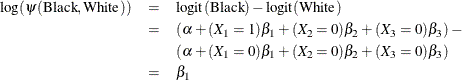
For the effect parameterization scheme (PARAM=EFFECT) with White as the reference group (REF=’White’), the design variables for Race are as follows:
|
Design Variables |
|||
|---|---|---|---|
|
Race |
|
|
|
|
Black |
1 |
0 |
0 |
|
Hispanic |
0 |
1 |
0 |
|
Other |
0 |
0 |
1 |
|
White |
–1 |
–1 |
–1 |
The log odds for Black is
The log odds for White is
Therefore, the log odds ratio of Black versus White becomes
For the reference cell parameterization scheme (PARAM=REF) with White as the reference cell, the design variables for race are as follows:
|
Design Variables |
|||
|---|---|---|---|
|
Race |
|
|
|
|
Black |
1 |
0 |
0 |
|
Hispanic |
0 |
1 |
0 |
|
Other |
0 |
0 |
1 |
|
White |
0 |
0 |
0 |
The log odds ratio of Black versus White is given by
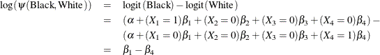
For the GLM parameterization scheme (PARAM=GLM), the design variables are as follows:
|
Design Variables |
||||
|---|---|---|---|---|
|
Race |
|
|
|
|
|
Black |
1 |
0 |
0 |
0 |
|
Hispanic |
0 |
1 |
0 |
0 |
|
Other |
0 |
0 |
1 |
0 |
|
White |
0 |
0 |
0 |
1 |
The log odds ratio of Black versus White is
Consider the hypothetical example of heart disease among race in Hosmer and Lemeshow (2000, p. 56). The entries in the following contingency table represent counts:
|
Race |
||||
|---|---|---|---|---|
|
Disease Status |
White |
Black |
Hispanic |
Other |
|
Present |
5 |
20 |
15 |
10 |
|
Absent |
20 |
10 |
10 |
10 |
The computation of odds ratio of Black versus White for various parameterization schemes is tabulated in Table 58.11.
Table 58.11: Odds Ratio of Heart Disease Comparing Black to White
|
Parameter Estimates |
|||||
|---|---|---|---|---|---|
|
PARAM= |
|
|
|
|
Odds Ratio Estimates |
|
EFFECT |
0.7651 |
0.4774 |
0.0719 |
|
|
|
REF |
2.0794 |
1.7917 |
1.3863 |
|
|
|
GLM |
2.0794 |
1.7917 |
1.3863 |
0.0000 |
|
Since the log odds ratio (![]() ) is a linear function of the parameters, the Wald confidence interval for
) is a linear function of the parameters, the Wald confidence interval for ![]() can be derived from the parameter estimates and the estimated covariance matrix. Confidence intervals for the odds ratios
are obtained by exponentiating the corresponding confidence limits for the log odd ratios. In the displayed output of PROC
LOGISTIC, the “Odds Ratio Estimates” table contains the odds ratio estimates and the corresponding 95% Wald confidence intervals. For continuous explanatory variables,
these odds ratios correspond to a unit increase in the risk factors.
can be derived from the parameter estimates and the estimated covariance matrix. Confidence intervals for the odds ratios
are obtained by exponentiating the corresponding confidence limits for the log odd ratios. In the displayed output of PROC
LOGISTIC, the “Odds Ratio Estimates” table contains the odds ratio estimates and the corresponding 95% Wald confidence intervals. For continuous explanatory variables,
these odds ratios correspond to a unit increase in the risk factors.
To customize odds ratios for specific units of change for a continuous risk factor, you can use the UNITS statement to specify a list of relevant units for each explanatory variable in the model. Estimates of these customized odds
ratios are given in a separate table. Let ![]() be a confidence interval for
be a confidence interval for ![]() . The corresponding lower and upper confidence limits for the customized odds ratio
. The corresponding lower and upper confidence limits for the customized odds ratio ![]() are
are ![]() and
and ![]() , respectively (for
, respectively (for ![]() ), or
), or ![]() and
and ![]() , respectively (for
, respectively (for ![]() ). You use the CLODDS= option or ODDSRATIO statement to request the confidence intervals for the odds ratios.
). You use the CLODDS= option or ODDSRATIO statement to request the confidence intervals for the odds ratios.
For a generalized logit model, odds ratios are computed similarly, except k odds ratios are computed for each effect, corresponding to the k logits in the model.