The GLMPOWER Procedure

Suppose you can enhance the planned study discussed in Example 46.1 in two ways:
-
incorporate results from races at two different altitudes (“high” and “low”)
-
measure the body mass index of each runner before the race
This is equivalent to adding a second fixed effect and a continuous covariate to your model.
Since lactic acid buildup is more pronounced at higher altitudes, you will include altitude as a factor in the model along with fluid, extending the one-way ANOVA to a two-way ANOVA. In doing so, you expect to lower the residual standard deviation from about 3.75 to 3.5 (in addition to generalizing the study results). You assume there is negligible interaction between fluid and altitude and plan to use a main-effects-only model. You conjecture that the mean lactic acid buildup follows Table 46.11.
Table 46.11: Mean Lactic Acid Buildup by Fluid and Altitude
|
Fluid |
|||||
|---|---|---|---|---|---|
|
Altitude |
Water |
EZD1 |
EZD2 |
LZ1 |
LZ2 |
|
High |
36.9 |
35.0 |
31.5 |
30 |
27.1 |
|
Low |
34.3 |
32.4 |
28.9 |
27 |
24.7 |
By including a measurement of body mass index as a covariate in the study, you hope to further reduce the error variability. The extent of this reduction in variability is commonly expressed in two alternative ways: (1) the correlation between the covariates and the response or (2) the proportional reduction in total R square incurred by the covariates. You prefer the former and guess that the correlation between body mass index and lactic acid buildup is between 0.2 and 0.3. You specify these estimates with the NCOVARIATES= and CORRXY= options in the POWER statement. The covariate is not included in the MODEL statement.
You are interested in the same four fluid comparisons as in Example 46.1, shown in Table 46.10, except this time you want to marginalize over the effect of altitude.
For each of these contrasts, you want to determine the sample size required to achieve a power of 0.9 to detect an effect
with magnitude according to Table 46.11. You are not yet attempting to choose a single sample size for the study, but rather checking the range of sample sizes needed
by individual contrasts. You plan to test each contrast at ![]() . You will provide twice as many runners with water as with any of the electrolytes, and you predict that you can study approximately
two-thirds as many runners at high altitude than at low altitude. The resulting planned sample size weighting scheme is shown
in Table 46.12. Since the scheme is only approximate, you use the NFRACTIONAL option in the POWER statement to disable the rounding of sample sizes up to integers satisfying the weights exactly.
. You will provide twice as many runners with water as with any of the electrolytes, and you predict that you can study approximately
two-thirds as many runners at high altitude than at low altitude. The resulting planned sample size weighting scheme is shown
in Table 46.12. Since the scheme is only approximate, you use the NFRACTIONAL option in the POWER statement to disable the rounding of sample sizes up to integers satisfying the weights exactly.
Table 46.12: Approximate Sample Size Allocation Weights
|
Fluid |
|||||
|---|---|---|---|---|---|
|
Altitude |
Water |
EZD1 |
EZD2 |
LZ1 |
LZ2 |
|
High |
4 |
2 |
2 |
2 |
2 |
|
Low |
6 |
3 |
3 |
3 |
3 |
First, you create the exemplary data set to specify means and weights for the design profiles:
data Fluids2;
   input Altitude $ Fluid $ LacticAcid CellWgt;
   datalines;
         High       Water      36.9       4
         High       EZD1       35.0       2
         High       EZD2       31.5       2
         High       LZ1        30         2
         High       LZ2        27.1       2
         Low        Water      34.3       6
         Low        EZD1       32.4       3
         Low        EZD2       28.9       3
         Low        LZ1        27         3
         Low        LZ2        24.7       3
;
The variables Altitude, Fluid, and LacticAcid specify the factors and cell means in Table 46.11. The variable CellWgt contains the sample size allocation weights in Table 46.12.
Use the DATA= option in the PROC GLMPOWER statement to specify Fluids2 as the exemplary data set. The following statements perform the sample size analysis:
proc glmpower data=Fluids2;
   class Altitude Fluid;
   model LacticAcid = Altitude Fluid;
   weight CellWgt;
   contrast "Water vs. others" Fluid  -1 -1 -1 -1 4;
   contrast "EZD vs. LZ"       Fluid   1  1 -1 -1 0;
   contrast "EZD1 vs. EZD2"    Fluid   1 -1  0  0 0;
   contrast "LZ1 vs. LZ2"      Fluid   0  0  1 -1 0;
   power
      nfractional
      stddev      = 3.5
      ncovariates = 1
      corrxy      = 0.2 0.3 0
      alpha       = 0.025
      ntotal      = .
      power       = 0.9;
run;
The CLASS statement identifies Altitude and Fluid as classification variables. The MODEL statement specifies the model, and the WEIGHT statement identifies CellWgt as the weight variable. The CONTRAST statement specifies the contrasts in Table 46.10. As in Example 46.1, the order of the contrast coefficients corresponds to the formatted class levels (EZD1, EZD2, LZ1, LZ2, Water). The POWER statement specifies total sample size as the result parameter and provides values for the other analysis parameters. The
NCOVARIATES= option specifies the single covariate (body mass index), and the CORRXY= option specifies the two scenarios for its correlation with lactic acid buildup (0.2 and 0.3). Output 46.2.1 displays the results.
Output 46.2.1: Sample Sizes for Two-Way ANOVA Contrasts
| Fixed Scenario Elements | |
|---|---|
| Dependent Variable | LacticAcid |
| Weight Variable | CellWgt |
| Alpha | 0.025 |
| Number of Covariates | 1 |
| Std Dev Without Covariate Adjustment | 3.5 |
| Nominal Power | 0.9 |
| Computed Ceiling N Total | |||||||||
|---|---|---|---|---|---|---|---|---|---|
| Index | Type | Source | Corr XY | Adj Std Dev | Test DF | Error DF | Fractional N Total | Actual Power | Ceiling N Total |
| 1 | Effect | Altitude | 0.2 | 3.43 | 1 | 84 | 90.418451 | 0.902 | 91 |
| 2 | Effect | Altitude | 0.3 | 3.34 | 1 | 79 | 85.862649 | 0.901 | 86 |
| 3 | Effect | Altitude | 0.0 | 3.50 | 1 | 88 | 94.063984 | 0.903 | 95 |
| 4 | Effect | Fluid | 0.2 | 3.43 | 4 | 16 | 22.446173 | 0.912 | 23 |
| 5 | Effect | Fluid | 0.3 | 3.34 | 4 | 15 | 21.687544 | 0.908 | 22 |
| 6 | Effect | Fluid | 0.0 | 3.50 | 4 | 17 | 23.055716 | 0.919 | 24 |
| 7 | Contrast | Water vs. others | 0.2 | 3.43 | 1 | 15 | 21.720195 | 0.905 | 22 |
| 8 | Contrast | Water vs. others | 0.3 | 3.34 | 1 | 14 | 20.848805 | 0.903 | 21 |
| 9 | Contrast | Water vs. others | 0.0 | 3.50 | 1 | 16 | 22.422381 | 0.910 | 23 |
| 10 | Contrast | EZD vs. LZ | 0.2 | 3.43 | 1 | 35 | 41.657424 | 0.903 | 42 |
| 11 | Contrast | EZD vs. LZ | 0.3 | 3.34 | 1 | 33 | 39.674037 | 0.903 | 40 |
| 12 | Contrast | EZD vs. LZ | 0.0 | 3.50 | 1 | 37 | 43.246415 | 0.906 | 44 |
| 13 | Contrast | EZD1 vs. EZD2 | 0.2 | 3.43 | 1 | 139 | 145.613657 | 0.901 | 146 |
| 14 | Contrast | EZD1 vs. EZD2 | 0.3 | 3.34 | 1 | 132 | 138.173983 | 0.902 | 139 |
| 15 | Contrast | EZD1 vs. EZD2 | 0.0 | 3.50 | 1 | 145 | 151.565917 | 0.901 | 152 |
| 16 | Contrast | LZ1 vs. LZ2 | 0.2 | 3.43 | 1 | 268 | 274.055008 | 0.901 | 275 |
| 17 | Contrast | LZ1 vs. LZ2 | 0.3 | 3.34 | 1 | 253 | 259.919126 | 0.900 | 260 |
| 18 | Contrast | LZ1 vs. LZ2 | 0.0 | 3.50 | 1 | 279 | 285.363976 | 0.901 | 286 |
The sample sizes in Output 46.2.1 range from 21 for the comparison of water versus electrolytes (assuming a correlation of 0.3 between body mass and lactic
acid buildup) to 275 for the comparison of LZ1 versus LZ2 (assuming a correlation of 0.2). PROC GLMPOWER also includes the
effect tests for Altitude and Fluid. Note that the required sample sizes for this study are lower than those for the study in Example 46.1.
Note that the error standard deviation has been reduced from 3.5 to 3.43 (when correlation is 0.2) or 3.34 (when correlation is 0.3) in the approximation of the effect of the body mass index covariate. The error degrees of freedom has also been automatically adjusted, lowered by 1 (the number of covariates).
Suppose you want to plot the required sample size for the range of power values from 0.5 to 0.95. First, define the analysis by specifying the same statements as before, but add the PLOTONLY option to the PROC GLMPOWER statement to disable the nongraphical results. Next, specify the PLOT statement with X=POWER to request a plot with power on the X axis. Sample size is automatically placed on the Y axis. Use the MIN= and MAX= options in the PLOT statement to specify the power range. The following statements produce the plot:
ods graphics on;

proc glmpower data=Fluids2 plotonly;
   class Altitude Fluid;
   model LacticAcid = Altitude Fluid;
   weight CellWgt;
   contrast "Water vs. others" Fluid  -1 -1 -1 -1 4;
   contrast "EZD vs. LZ"       Fluid   1  1 -1 -1 0;
   contrast "EZD1 vs. EZD2"    Fluid   1 -1  0  0 0;
   contrast "LZ1 vs. LZ2"      Fluid   0  0  1 -1 0;
   power
      nfractional
      stddev      = 3.5
      ncovariates = 1
      corrxy      = 0.2 0.3 0
      alpha       = 0.025
      ntotal      = .
      power       = 0.9;
   plot x=power min=.5 max=.95;
run;
See Output 46.2.2 for the resulting plot.
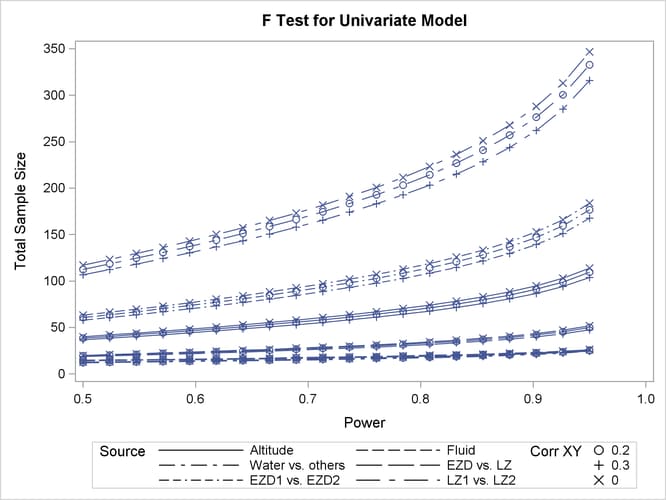
In Output 46.1.2, the line style identifies the test, and the plotting symbol identifies the scenario for the correlation between covariate and response. The plotting symbol locations identify actual computed powers; the curves are linear interpolations of these points. As in Example 46.1, the required sample size is highest for the test of LZ1 versus LZ2.
Finally, suppose you want to plot the power for the range of sample sizes you will likely consider for the study (the range of 21 to 275 that achieves 0.9 power for different comparisons). In the POWER statement, identify power as the result (POWER=.), and specify NTOTAL=21. Specify the PLOT statement with X=N to request a plot with sample size on the X axis.
The following statements produce the plot:
proc glmpower data=Fluids2 plotonly;
   class Altitude Fluid;
   model LacticAcid = Altitude Fluid;
   weight CellWgt;
   contrast "Water vs. others" Fluid  -1 -1 -1 -1 4;
   contrast "EZD vs. LZ"       Fluid   1  1 -1 -1 0;
   contrast "EZD1 vs. EZD2"    Fluid   1 -1  0  0 0;
   contrast "LZ1 vs. LZ2"      Fluid   0  0  1 -1 0;
   power
      nfractional
      stddev      = 3.5
      ncovariates = 1
      corrxy      = 0.2 0.3 0
      alpha       = 0.025
      ntotal      = 21
      power       = .;
   plot x=n min=21 max=275;
run;

ods graphics off;
The MAX=275 option in the PLOT statement sets the maximum sample size value. The MIN= option automatically defaults to the value of 21 from the NTOTAL= option in the POWER statement.
See Output 46.2.3 for the plot.

Although Output 46.2.2 and Output 46.2.3 surface essentially the same computations for practical power ranges, they each provide a different quick visual assessment. Output 46.2.2 reveals the range of required sample sizes for powers of interest, and Output 46.2.3 reveals the range of powers achieved for sample sizes of interest.