The GLMPOWER Procedure

This example deals with the same situation as in Example 75.1 in Chapter 75: The POWER Procedure.
Hocking (1985, p. 109) describes a study of the effectiveness of electrolytes in reducing lactic acid buildup for long-distance runners. You are planning a similar study in which you will allocate five different fluids to runners on a 10-mile course and measure lactic acid buildup immediately after the race. The fluids consist of water and two commercial electrolyte drinks, EZDure and LactoZap, each prepared at two concentrations, low (EZD1 and LZ1) and high (EZD2 and LZ2).
You conjecture that the standard deviation of lactic acid measurements given any particular fluid is about 3.75, and that the expected lactic acid values will correspond roughly to Table 46.9. You are least familiar with the LZ1 drink and hence decide to consider a range of reasonable values for that mean.
You are interested in four different comparisons, shown in Table 46.10 with appropriate contrast coefficients.
Table 46.10: Planned Comparisons
|
Contrast Coefficients |
|||||
|---|---|---|---|---|---|
|
Comparison |
Water |
EZD1 |
EZD2 |
LZ1 |
LZ2 |
|
Water versus electrolytes |
4 |
-1 |
-1 |
-1 |
-1 |
|
EZD versus LZ |
0 |
1 |
1 |
-1 |
-1 |
|
EZD1 versus EZD2 |
0 |
1 |
-1 |
0 |
0 |
|
LZ1 versus LZ2 |
0 |
0 |
0 |
1 |
-1 |
For each of these contrasts you want to determine the sample size required to achieve a power of 0.9 for detecting an effect
with magnitude in accord with Table 46.9. You are not yet attempting to choose a single sample size for the study, but rather checking the range of sample sizes needed
for individual contrasts. You plan to test each contrast at ![]() . In the interests of reducing costs, you will provide twice as many runners with water as with any of the electrolytes; that
is, you will use a sample size weighting scheme of 2:1:1:1:1.
. In the interests of reducing costs, you will provide twice as many runners with water as with any of the electrolytes; that
is, you will use a sample size weighting scheme of 2:1:1:1:1.
Before calling PROC GLMPOWER, you need to create the exemplary data set to specify means and weights for the design profiles:
data Fluids;
   input Fluid $ LacticAcid1 LacticAcid2 CellWgt;
   datalines;
         Water      35.6        35.6        2
         EZD1       33.7        33.7        1
         EZD2       30.2        30.2        1
         LZ1        29          28          1
         LZ2        25.9        25.9        1
;
The variable LacticAcid1 represents the cell means scenario with the larger LZ1 mean (29), and LacticAcid2 represents the scenario with the smaller LZ1 mean (28). The variable CellWgt contains the sample size allocation weights.
Use the DATA= option in the PROC GLMPOWER statement to specify Fluids as the exemplary data set. The following statements perform the sample size analysis:
proc glmpower data=Fluids;
   class Fluid;
   model LacticAcid1 LacticAcid2 = Fluid;
   weight CellWgt;
   contrast "Water vs. others" Fluid  -1 -1 -1 -1 4;
   contrast "EZD vs. LZ"       Fluid   1  1 -1 -1 0;
   contrast "EZD1 vs. EZD2"    Fluid   1 -1  0  0 0;
   contrast "LZ1 vs. LZ2"      Fluid   0  0  1 -1 0;
   power
      stddev = 3.75
      alpha  = 0.025
      ntotal = .
      power  = 0.9;
run;
The CLASS statement identifies Fluid as a classification variable. The MODEL statement specifies the model and the two cell means scenarios LacticAcid1 and LacticAcid2. The WEIGHT statement identifies CellWgt as the weight variable. The CONTRAST statement specifies the contrasts. Since PROC GLMPOWER by default processes class levels in order of formatted values, the
contrast coefficients correspond to the following order: EZD1, EZD2, LZ1, LZ2, Water. (
Note: You could use the ORDER=DATA option in the PROC GLMPOWER statement to achieve the same ordering as in Table 46.10 instead.) The POWER statement specifies total sample size as the result parameter and provides values for the other analysis parameters (error
standard deviation, alpha, and power).
Output 46.1.1 displays the results.
Output 46.1.1: Sample Sizes for One-Way ANOVA Contrasts
| Fixed Scenario Elements | |
|---|---|
| Weight Variable | CellWgt |
| Alpha | 0.025 |
| Error Standard Deviation | 3.75 |
| Nominal Power | 0.9 |
| Computed N Total | |||||||
|---|---|---|---|---|---|---|---|
| Index | Dependent | Type | Source | Test DF | Error DF | Actual Power | N Total |
| 1 | LacticAcid1 | Effect | Fluid | 4 | 25 | 0.958 | 30 |
| 2 | LacticAcid1 | Contrast | Water vs. others | 1 | 25 | 0.947 | 30 |
| 3 | LacticAcid1 | Contrast | EZD vs. LZ | 1 | 55 | 0.929 | 60 |
| 4 | LacticAcid1 | Contrast | EZD1 vs. EZD2 | 1 | 169 | 0.901 | 174 |
| 5 | LacticAcid1 | Contrast | LZ1 vs. LZ2 | 1 | 217 | 0.902 | 222 |
| 6 | LacticAcid2 | Effect | Fluid | 4 | 25 | 0.972 | 30 |
| 7 | LacticAcid2 | Contrast | Water vs. others | 1 | 19 | 0.901 | 24 |
| 8 | LacticAcid2 | Contrast | EZD vs. LZ | 1 | 43 | 0.922 | 48 |
| 9 | LacticAcid2 | Contrast | EZD1 vs. EZD2 | 1 | 169 | 0.901 | 174 |
| 10 | LacticAcid2 | Contrast | LZ1 vs. LZ2 | 1 | 475 | 0.902 | 480 |
The sample sizes range from 24 for the comparison of water versus electrolytes to 480 for the comparison of LZ1 versus LZ2,
both assuming the smaller LZ1 mean. The sample size for the latter comparison is relatively large because the small mean difference
of ![]() is hard to detect. PROC GLMPOWER also includes the effect test for
is hard to detect. PROC GLMPOWER also includes the effect test for Fluid. Note that, in this case, it is equivalent to TEST=OVERALL_F in the ONEWAYANOVA statement of PROC POWER, since there is only
one effect in the model.
The Nominal Power of 0.9 in the “Fixed Scenario Elements” table in Output 46.1.1 represents the input target power, and the Actual Power column in the “Computed N Total” table is the power at the sample size (N Total) adjusted to achieve the specified sample weighting. Note that all of the sample sizes are rounded up to multiples of 6 to preserve integer group sizes (since the group weights add up to 6). You can use the NFRACTIONAL option in the POWER statement to compute raw fractional sample sizes.
Suppose you want to plot the required sample size for the range of power values from 0.5 to 0.95. First, define the analysis by specifying the same statements as before, but add the PLOTONLY option to the PROC GLMPOWER statement to disable the nongraphical results. Next, specify the PLOT statement with X=POWER to request a plot with power on the X axis. (The result parameter—here sample size—is always plotted on the other axis.) Use the MIN= and MAX= options in the PLOT statement to specify the power range. The following statements produce the plot:
ods graphics on;

proc glmpower data=Fluids plotonly;
   class Fluid;
   model LacticAcid1 LacticAcid2 = Fluid;
   weight CellWgt;
   contrast "Water vs. others" Fluid  -1 -1 -1 -1 4;
   contrast "EZD vs. LZ"       Fluid   1  1 -1 -1 0;
   contrast "EZD1 vs. EZD2"    Fluid   1 -1  0  0 0;
   contrast "LZ1 vs. LZ2"      Fluid   0  0  1 -1 0;
   power
      stddev = 3.75
      alpha  = 0.025
      ntotal = .
      power  = 0.9;
   plot x=power min=.5 max=.95;
run;
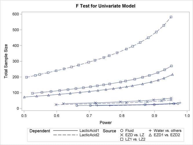
In Output 46.1.2, the line style identifies the cell means scenario, and the plotting symbol identifies the test. The plotting symbol locations identify actual computed powers; the curves are linear interpolations of these points. The plot shows that the required sample size is highest for the test of LZ1 versus LZ2, which was previously found to require the most resources.
Note that some of the plotted points in Output 46.1.2 are unevenly spaced. This is because the plotted points are the rounded sample size results at their corresponding actual power levels. The range specified with the MIN= and MAX= values in the PLOT statement corresponds to nominal power levels. In some cases, actual power is substantially higher than nominal power. To obtain plots with evenly spaced points (but with fractional sample sizes at the computed points), you can use the NFRACTIONAL option in the POWER statement preceding the PLOT statement.
Finally, suppose you want to plot the power for the range of sample sizes you will likely consider for the study (the range of 24 to 480 that achieves 0.9 power for different comparisons). In the POWER statement, identify power as the result (POWER=.), and specify any total sample size value (say, NTOTAL=100). Specify the PLOT statement with X=N to request a plot with sample size on the X axis.
The following statements produce the plot:
proc glmpower data=Fluids plotonly;
   class Fluid;
   model LacticAcid1 LacticAcid2 = Fluid;
   weight CellWgt;
   contrast "Water vs. others" Fluid  -1 -1 -1 -1 4;
   contrast "EZD vs. LZ"       Fluid   1  1 -1 -1 0;
   contrast "EZD1 vs. EZD2"    Fluid   1 -1  0  0 0;
   contrast "LZ1 vs. LZ2"      Fluid   0  0  1 -1 0;
   power
      stddev = 3.75
      alpha  = 0.025
      ntotal = 24
      power  = .;
   plot x=n min=24 max=480;
run;

ods graphics off;
Note that the value 100 specified with the NTOTAL=100 option is not used. It is overridden in the plot by the MIN= and MAX= options in the PLOT statement, and the PLOTONLY option in the PROC GLMPOWER statement disables nongraphical results. But the NTOTAL= option (along with a value) is still needed in the POWER statement as a placeholder, to identify the desired parameterization for sample size.
See Output 46.1.3 for the plot.
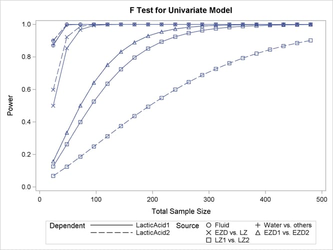
Although Output 46.1.2 and Output 46.1.3 surface essentially the same computations for practical power ranges, they each provide a different quick visual assessment. Output 46.1.2 reveals the range of required sample sizes for powers of interest, and Output 46.1.3 reveals the range of achieved powers for sample sizes of interest.