The SEQDESIGN Procedure
-
Overview

- Getting Started
-
Syntax
-
DetailsFixed-Sample Clinical TrialsOne-Sided Fixed-Sample Tests in Clinical TrialsTwo-Sided Fixed-Sample Tests in Clinical TrialsGroup Sequential MethodsStatistical Assumptions for Group Sequential DesignsBoundary ScalesBoundary VariablesType I and Type II ErrorsUnified Family MethodsHaybittle-Peto MethodWhitehead MethodsError Spending MethodsAcceptance (beta) BoundaryBoundary Adjustments for Overlapping Lower and Upper beta BoundariesSpecified and Derived ParametersApplicable Boundary KeysSample Size ComputationApplicable One-Sample Tests and Sample Size ComputationApplicable Two-Sample Tests and Sample Size ComputationApplicable Regression Parameter Tests and Sample Size ComputationAspects of Group Sequential DesignsSummary of Methods in Group Sequential DesignsTable OutputODS Table NamesGraphics OutputODS Graphics
-
ExamplesCreating Fixed-Sample DesignsCreating a One-Sided O’Brien-Fleming DesignCreating Two-Sided Pocock and O’Brien-Fleming DesignsGenerating Graphics Display for Sequential DesignsCreating Designs Using Haybittle-Peto MethodsCreating Designs with Various Stopping CriteriaCreating Whitehead’s Triangular DesignsCreating a One-Sided Error Spending DesignCreating Designs with Various Number of StagesCreating Two-Sided Error Spending Designs with and without Overlapping Lower and Upper beta BoundariesCreating a Two-Sided Asymmetric Error Spending Design with Early Stopping to Reject H0Creating a Two-Sided Asymmetric Error Spending Design with Early Stopping to Reject or Accept H0Creating a Design with a Nonbinding Beta BoundaryComputing Sample Size for Survival Data
- References
This example requests two three-stage group sequential designs for normally distributed statistics. Each design uses a power
family error spending function with a specified two-sided alternative hypothesis ![]() and early stopping only to accept the null hypothesis
and early stopping only to accept the null hypothesis ![]() .
.
The first design uses the BETAOVERLAP=NOADJUST option to derive acceptance boundary values without adjusting for the possible
overlapping of the lower and upper ![]() boundaries computed from the two corresponding one-sided tests. The second design uses the BETAOVERLAP=ADJUST option to test
the overlapping of the
boundaries computed from the two corresponding one-sided tests. The second design uses the BETAOVERLAP=ADJUST option to test
the overlapping of the ![]() boundaries at each interim stage based on the two corresponding one-sided tests and then to set the
boundaries at each interim stage based on the two corresponding one-sided tests and then to set the ![]() boundary values at the stage to missing if overlapping occurs at that stage.
boundary values at the stage to missing if overlapping occurs at that stage.
The following statements request a two-sided design with the BETAOVERLAP=NOADJUST option:
ods graphics on;
proc seqdesign altref=0.2 errspend;
   design nstages=3
          method=errfuncpow
          alt=twosided  stop=accept
          betaoverlap=noadjust
          beta=0.09
          ;
run;
ods graphics off;
The “Design Information” table in Output 83.10.1 displays design specifications and the derived statistics for the first design. With the specified alternative reference
![]() , the maximum information is derived.
, the maximum information is derived.
Output 83.10.1: Design Information
| Design Information | |
|---|---|
| Statistic Distribution | Normal |
| Boundary Scale | Standardized Z |
| Alternative Hypothesis | Two-Sided |
| Early Stop | Accept Null |
| Method | Error Spending |
| Boundary Key | Both |
| Alternative Reference | 0.2 |
| Number of Stages | 3 |
| Alpha | 0.05 |
| Beta | 0.09 |
| Power | 0.91 |
| Max Information (Percent of Fixed Sample) | 103.8789 |
| Max Information | 282.9328 |
| Null Ref ASN (Percent of Fixed Sample) | 79.20197 |
| Alt Ref ASN (Percent of Fixed Sample) | 102.1476 |
The “Boundary Information” table in Output 83.10.2 displays the information level, alternative reference, and boundary values. With a specified alternative reference ![]() , the maximum information is derived from the procedure, and the actual information level at each stage is displayed in the
table. By default (or equivalently if you specify BOUNDARYSCALE=STDZ), the alternative reference and boundary values are displayed
with the standardized Z scale. The alternative reference at stage k is given by
, the maximum information is derived from the procedure, and the actual information level at each stage is displayed in the
table. By default (or equivalently if you specify BOUNDARYSCALE=STDZ), the alternative reference and boundary values are displayed
with the standardized Z scale. The alternative reference at stage k is given by ![]() , where
, where ![]() is the specified alternative reference and
is the specified alternative reference and ![]() is the information level at stage k,
is the information level at stage k, ![]() .
.
Output 83.10.2: Boundary Information
| Boundary Information (Standardized Z Scale) Null Reference = 0 |
||||||
|---|---|---|---|---|---|---|
| _Stage_ | Alternative | Boundary Values | ||||
| Information Level | Reference | Lower | Upper | |||
| Proportion | Actual | Lower | Upper | Beta | Beta | |
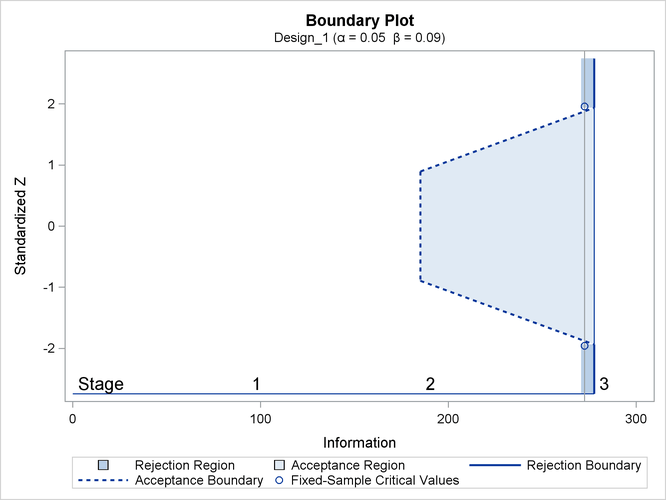
| 1 | 0.3333 | 94.31094 | -1.94228 | 1.94228 | -0.08239 | 0.08239 |
| 2 | 0.6667 | 188.6219 | -2.74679 | 2.74679 | -0.90351 | 0.90351 |
| 3 | 1.0000 | 282.9328 | -3.36412 | 3.36412 | -1.92519 | 1.92519 |
The “Error Spending Information” table in Output 83.10.3 displays the cumulative error spending at each stage for each boundary.
Output 83.10.3: Error Spending Information
| Error Spending Information | |||||
|---|---|---|---|---|---|
| _Stage_ | Information Level |
Cumulative Error Spending | |||
| Lower | Upper | ||||
| Proportion | Alpha | Beta | Beta | Alpha | |
| 1 | 0.3333 | 0.00000 | 0.01000 | 0.01000 | 0.00000 |
| 2 | 0.6667 | 0.00000 | 0.04000 | 0.04000 | 0.00000 |
| 3 | 1.0000 | 0.02500 | 0.09000 | 0.09000 | 0.02500 |
With the STOP=ACCEPT option, the design does not stop at interim stages to reject ![]() , and the
, and the ![]() spending at each interim stage is zero. For the power family error spending function with the default parameter
spending at each interim stage is zero. For the power family error spending function with the default parameter ![]() , the beta spending at stage 1 is
, the beta spending at stage 1 is ![]() , and the cumulative beta spending at stage 2 is
, and the cumulative beta spending at stage 2 is ![]() .
.
With ODS Graphics enabled, a detailed boundary plot with the acceptance and rejection regions is displayed, as shown in Output 83.10.4.
The following statements request a two-sided design with the BETAOVERLAP=ADJUST option, which is the default:
ods graphics on;
proc seqdesign altref=0.2 errspend;
   design nstages=3
          method=errfuncpow
          alt=twosided
          stop=accept
          betaoverlap=adjust
          beta=0.09
          ;
run;
ods graphics off;
With the BETAOVERLAP=ADJUST option, the procedure first derives the usual ![]() boundary values for the two-sided design and then checks for overlapping of the
boundary values for the two-sided design and then checks for overlapping of the ![]() boundaries for the two corresponding one-sided tests at each stage. If this type of overlapping occurs at a particular stage,
the
boundaries for the two corresponding one-sided tests at each stage. If this type of overlapping occurs at a particular stage,
the ![]() boundary values for that stage are set to missing, the
boundary values for that stage are set to missing, the ![]() spending values at that stage are reset to zero, and the
spending values at that stage are reset to zero, and the ![]() spending values at subsequent stages are adjusted proportionally.
spending values at subsequent stages are adjusted proportionally.
The boundary values without adjusting for the possible overlapping of the two one-sided ![]() boundaries are identical to the boundary values derived in the first design (with the BETAOVERLAP=NOADJUST option, as shown
in Output 83.10.2). At stage 1, the upper
boundaries are identical to the boundary values derived in the first design (with the BETAOVERLAP=NOADJUST option, as shown
in Output 83.10.2). At stage 1, the upper ![]() boundary value for the corresponding one-sided test is
boundary value for the corresponding one-sided test is
where ![]() is the upper alternative reference,
is the upper alternative reference, ![]() is the information level at stage 1, and
is the information level at stage 1, and ![]() is the
is the ![]() spending at stage 1 (as shown in Output 83.10.3).
spending at stage 1 (as shown in Output 83.10.3).
Similarly, the lower ![]() boundary value for the corresponding one-sided test is computed as 0.38407. Since the upper
boundary value for the corresponding one-sided test is computed as 0.38407. Since the upper ![]() boundary value is less than the lower
boundary value is less than the lower ![]() boundary at stage 1, overlapping occurs, and so the
boundary at stage 1, overlapping occurs, and so the ![]() boundary values for the two-sided design are set to missing at stage 1.
boundary values for the two-sided design are set to missing at stage 1.
With the ![]() boundary values set to missing at stage 1 and the
boundary values set to missing at stage 1 and the ![]() spending
spending ![]() the
the ![]() spending values at subsequent interim stages are adjusted proportionally. In this example, the adjusted
spending values at subsequent interim stages are adjusted proportionally. In this example, the adjusted ![]() spending at stage 2 is computed as
spending at stage 2 is computed as
where ![]() is the cumulative
is the cumulative ![]() spending at stage k before the adjustment,
spending at stage k before the adjustment, ![]() .
.
The “Design Information” table in Output 83.10.5 displays design specifications and derived statistics for the design.
Output 83.10.5: Design Information
| Design Information | |
|---|---|
| Statistic Distribution | Normal |
| Boundary Scale | Standardized Z |
| Alternative Hypothesis | Two-Sided |
| Early Stop | Accept Null |
| Method | Error Spending |
| Boundary Key | Both |
| Alternative Reference | 0.2 |
| Number of Stages | 3 |
| Alpha | 0.05 |
| Beta | 0.09 |
| Power | 0.91 |
| Max Information (Percent of Fixed Sample) | 101.9388 |
| Max Information | 277.649 |
| Null Ref ASN (Percent of Fixed Sample) | 80.56408 |
| Alt Ref ASN (Percent of Fixed Sample) | 100.792 |
The “Boundary Information” table in Output 83.10.6 displays the information levels, alternative references, and boundary values.
Output 83.10.6: Boundary Information
| Boundary Information (Standardized Z Scale) Null Reference = 0 |
||||||
|---|---|---|---|---|---|---|
| _Stage_ | Alternative | Boundary Values | ||||
| Information Level | Reference | Lower | Upper | |||
| Proportion | Actual | Lower | Upper | Beta | Beta | |
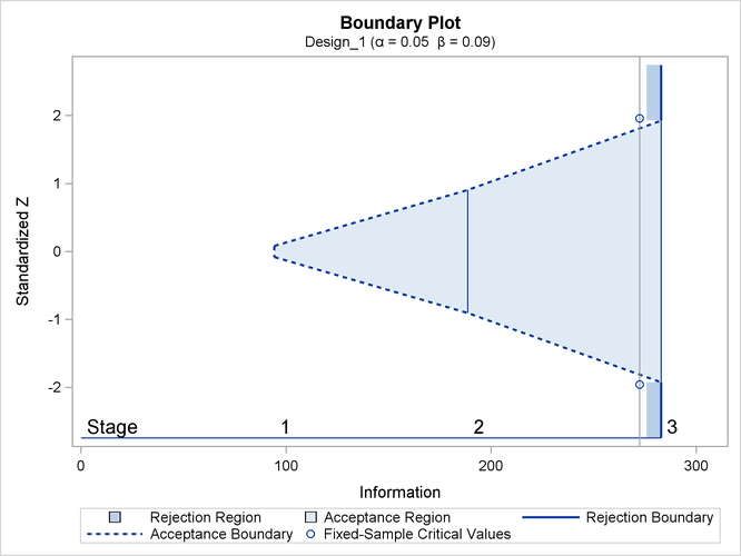
| 1 | 0.3333 | 92.54967 | -1.92405 | 1.92405 | . | . |
| 2 | 0.6667 | 185.0993 | -2.72102 | 2.72102 | -0.89469 | 0.89469 |
| 3 | 1.0000 | 277.649 | -3.33256 | 3.33256 | -1.93494 | 1.93494 |
The “Error Spending Information” table in Output 83.10.7 displays the cumulative error spending at each stage for each boundary.
Output 83.10.7: Error Spending Information
| Error Spending Information | |||||
|---|---|---|---|---|---|
| _Stage_ | Information Level |
Cumulative Error Spending | |||
| Lower | Upper | ||||
| Proportion | Alpha | Beta | Beta | Alpha | |
| 1 | 0.3333 | 0.00000 | 0.00000 | 0.00000 | 0.00000 |
| 2 | 0.6667 | 0.00000 | 0.03375 | 0.03375 | 0.00000 |
| 3 | 1.0000 | 0.02500 | 0.09000 | 0.09000 | 0.02500 |
With ODS Graphics enabled, a detailed boundary plot with the acceptance and rejection regions is displayed, as shown in Output 83.10.8.