The SEQDESIGN Procedure
-
Overview

- Getting Started
-
Syntax
-
DetailsFixed-Sample Clinical TrialsOne-Sided Fixed-Sample Tests in Clinical TrialsTwo-Sided Fixed-Sample Tests in Clinical TrialsGroup Sequential MethodsStatistical Assumptions for Group Sequential DesignsBoundary ScalesBoundary VariablesType I and Type II ErrorsUnified Family MethodsHaybittle-Peto MethodWhitehead MethodsError Spending MethodsAcceptance (beta) BoundaryBoundary Adjustments for Overlapping Lower and Upper beta BoundariesSpecified and Derived ParametersApplicable Boundary KeysSample Size ComputationApplicable One-Sample Tests and Sample Size ComputationApplicable Two-Sample Tests and Sample Size ComputationApplicable Regression Parameter Tests and Sample Size ComputationAspects of Group Sequential DesignsSummary of Methods in Group Sequential DesignsTable OutputODS Table NamesGraphics OutputODS Graphics
-
ExamplesCreating Fixed-Sample DesignsCreating a One-Sided O’Brien-Fleming DesignCreating Two-Sided Pocock and O’Brien-Fleming DesignsGenerating Graphics Display for Sequential DesignsCreating Designs Using Haybittle-Peto MethodsCreating Designs with Various Stopping CriteriaCreating Whitehead’s Triangular DesignsCreating a One-Sided Error Spending DesignCreating Designs with Various Number of StagesCreating Two-Sided Error Spending Designs with and without Overlapping Lower and Upper beta BoundariesCreating a Two-Sided Asymmetric Error Spending Design with Early Stopping to Reject H0Creating a Two-Sided Asymmetric Error Spending Design with Early Stopping to Reject or Accept H0Creating a Design with a Nonbinding Beta BoundaryComputing Sample Size for Survival Data
- References
This example creates the same group sequential design as in Example 83.3 and creates graphics by using ODS Graphics. The following statements request all available graphs in the SEQDESIGN procedure:
ods graphics on;
proc seqdesign altref=0.4
               plots=all
               ;
   TwoSidedPocock:        design nstages=4 method=poc;
   TwoSidedOBrienFleming: design nstages=4 method=obf;
run;
ods graphics off;
With the PLOTS=ALL option, a detailed boundary plot with the rejection region and acceptance region is displayed for the Pocock design, as shown in Output 83.4.1. By default (or equivalently if you specify STOP=REJECT), the rejection boundaries are also generated at interim stages.
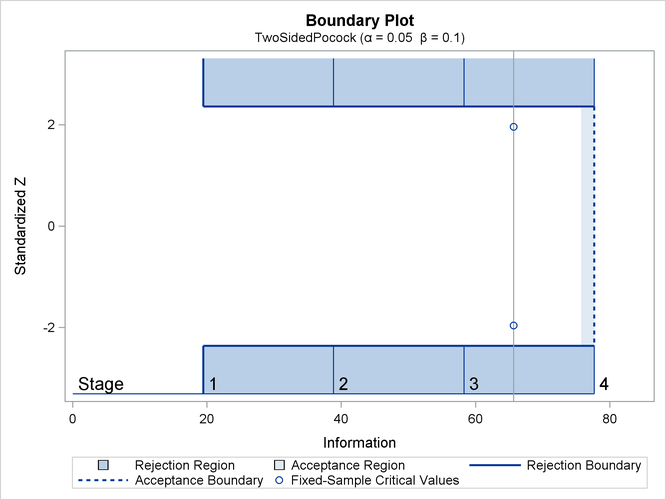
The plot shows identical boundary values in each boundary in the standardized Z scale for the Pocock design. The information level and the critical value for the corresponding fixed-sample design are also displayed.
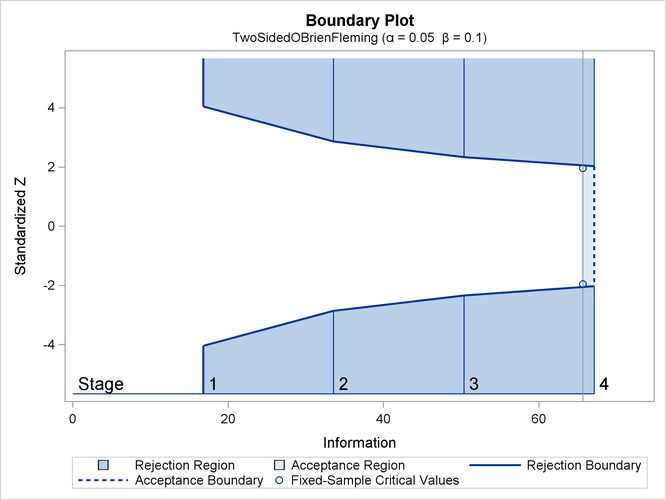
With the PLOTS=ALL option, a detailed boundary plot with the rejection region and acceptance region is also displayed for the O’Brien-Fleming design, as shown in Output 83.4.2. The plot shows that the rejection boundary values are decreasing as the trial advances in the standardized Z scale.
With the PLOTS=ALL option, the procedure displays a plot of average sample numbers (expected sample sizes for nonsurvival
data or expected numbers of events for survival data) under various hypothetical references for all designs simultaneously,
as shown in Output 83.4.3. By default, the option CREF= ![]() and expected sample sizes under the hypothetical references
and expected sample sizes under the hypothetical references ![]() are displayed, where
are displayed, where ![]() are values specified in the CREF= option. These CREF= values are displayed on the horizontal axis.
are values specified in the CREF= option. These CREF= values are displayed on the horizontal axis.
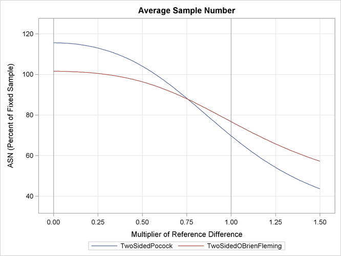
The plot shows that the Pocock design has a larger expected sample size than the O’Brien-Fleming design under the null hypothesis
(![]() ) and has a smaller expected sample size under the alternative hypothesis (
) and has a smaller expected sample size under the alternative hypothesis (![]() ).
).
With the PLOTS=ALL option, the procedure displays a plot of the power curves under various hypothetical references for all
designs simultaneously, as shown in Output 83.4.4. By default, the option CREF= ![]() and powers under hypothetical references
and powers under hypothetical references ![]() are displayed, where
are displayed, where ![]() are values specified in the CREF= option. These CREF= values are displayed on the horizontal axis.
are values specified in the CREF= option. These CREF= values are displayed on the horizontal axis.
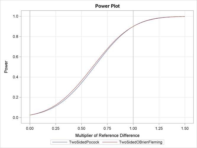
Under the null hypothesis, ![]() , the power is 0.025, the upper Type I error probability. Under the alternative hypothesis,
, the power is 0.025, the upper Type I error probability. Under the alternative hypothesis, ![]() , the power is 0.9, one minus the Type II error probability. The plot shows only minor difference between the two designs.
, the power is 0.9, one minus the Type II error probability. The plot shows only minor difference between the two designs.
With the PLOTS=ALL option, the procedure displays a plot of sequential boundaries for all designs simultaneously, as shown in Output 83.4.5. By default (or equivalently if you specify HSCALE=INFO in the COMBINEDBOUNDARY option), the information levels are used on the horizontal axis.
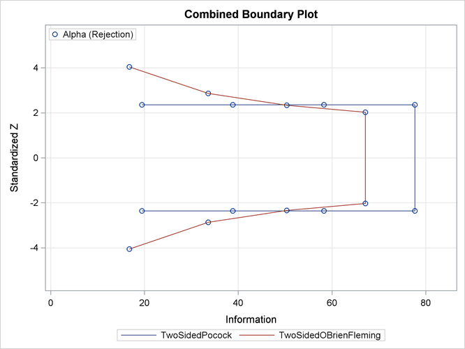
The plot shows that the ![]() boundary values (in absolute value) created from the O’Brien-Fleming method are greater in early stages and smaller in later
stages than the boundary values from the Pocock method. The plot also shows that the information level in the Pocock design
is larger than the corresponding level in the O’Brien-Fleming design at each stage.
boundary values (in absolute value) created from the O’Brien-Fleming method are greater in early stages and smaller in later
stages than the boundary values from the Pocock method. The plot also shows that the information level in the Pocock design
is larger than the corresponding level in the O’Brien-Fleming design at each stage.
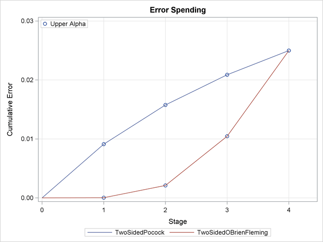
With the PLOTS=ALL option, the procedure displays a plot of cumulative error spends for all boundaries in the designs simultaneously,
as shown in Output 83.4.6. With a symmetric two-sided design, cumulative error spending is displayed only for the upper ![]() boundary. The plot shows that for the upper
boundary. The plot shows that for the upper ![]() boundary, the O’Brien-Fleming method spends fewer errors in early stages and more errors in later stages than the corresponding
Pocock method.
boundary, the O’Brien-Fleming method spends fewer errors in early stages and more errors in later stages than the corresponding
Pocock method.