The POWER Procedure
- Overview
-
Getting Started

-
Syntax
-
Details
-
ExamplesOne-Way ANOVAThe Sawtooth Power Function in Proportion AnalysesSimple AB/BA Crossover DesignsNoninferiority Test with Lognormal DataMultiple Regression and CorrelationComparing Two Survival CurvesConfidence Interval PrecisionCustomizing PlotsBinary Logistic Regression with Independent PredictorsWilcoxon-Mann-Whitney Test
- References
Crossover trials are experiments in which each subject is given a sequence of different treatments. They are especially common in clinical trials for medical studies. The reduction in variability from taking multiple measurements on a subject allows for more precise treatment comparisons. The simplest such design is the AB/BA crossover, in which each subject receives each of two treatments in a randomized order.
Under certain simplifying assumptions, you can test the treatment difference in an AB/BA crossover trial by using either a paired or two-sample t test (or equivalence test, depending on the hypothesis). This example will demonstrate when and how you can use the PAIREDMEANS statement in PROC POWER to perform power analyses for AB/BA crossover designs.
Senn (1993, Chapter 3) discusses a study comparing the effects of two bronchodilator medications in treatment of asthma, by using an AB/BA crossover design. Suppose you want to plan a similar study comparing two new medications, “Xilodol” and “Brantium.” Half of the patients would be assigned to sequence AB, getting a dose of Xilodol in the first treatment period, a wash-out period of one week, and then a dose of Brantium in the second treatment period. The other half would be assigned to sequence BA, following the same schedule but with the drugs reversed. In each treatment period you would administer the drugs in the morning and then measure peak expiratory flow (PEF) at the end of the day, with higher PEF representing better lung function.
You conjecture that the mean and standard deviation of PEF are about ![]() = 330 and
= 330 and ![]() = 40 for Xilodol and
= 40 for Xilodol and ![]() = 310 and
= 310 and ![]() = 55 for Brantium, and that each pair of measurements on the same subject will have a correlation of about 0.3. You want
to compute the power of both one-sided and two-sided tests of mean difference, with a significance level of
= 55 for Brantium, and that each pair of measurements on the same subject will have a correlation of about 0.3. You want
to compute the power of both one-sided and two-sided tests of mean difference, with a significance level of ![]() , for a sample size of 100 patients and also plot the power for a range of 50 to 200 patients. Note that the allocation ratio
of patients to the two sequences is irrelevant in this analysis.
, for a sample size of 100 patients and also plot the power for a range of 50 to 200 patients. Note that the allocation ratio
of patients to the two sequences is irrelevant in this analysis.
The choice of statistical test depends on which assumptions are reasonable. One possibility is a t test. A paired or two-sample t test is valid when there is no carryover effect and no interactions between patients, treatments, and periods. See Senn (1993, Chapter 3) for more details. The choice between a paired or a two-sample test depends on what you assume about the period effect. If you assume no period effect, then a paired t test is the appropriate analysis for the design, with the first member of each pair being the Xilodol measurement (regardless of which sequence the patient belongs to). Otherwise, the two-sample t test approach is called for, since this analysis adjusts for the period effect by using an extra degree of freedom.
Suppose you assume no period effect. Then you can use the PAIREDMEANS statement in PROC POWER with the TEST=DIFF option to perform a sample size analysis for the paired t test. Indicate power as the result parameter by specifying the POWER= option with a missing value (.). Specify the conjectured means and standard deviations for each drug by using the PAIREDMEANS= and PAIREDSTDDEVS= options and the correlation by using the CORR= option. Specify both one- and two-sided tests by using the SIDES= option, the significance level by using the ALPHA= option, and the sample size (in terms of number of pairs) by using the NPAIRS= option. Generate a plot of power versus sample size by specifying the PLOT statement with X=N to request a plot with sample size on the X axis. (The result parameter, here power, is always plotted on the other axis.) Use the MIN= and MAX= options in the PLOT statement to specify the sample size range (as numbers of pairs).
The following statements perform the sample size analysis:
ods listing style=htmlbluecml;
ods graphics on;

proc power;
   pairedmeans test=diff
      pairedmeans   = (330 310)
      pairedstddevs = (40 55)
      corr          = 0.3
      sides         = 1 2
      alpha         = 0.01
      npairs        = 100
      power         = .;
   plot x=n min=50 max=200;
run;

ods graphics off;
The ODS LISTING STYLE=HTMLBLUECML statement specifies the HTMLBLUECML style, which is suitable for use with PROC POWER because it allows both marker symbols and line styles to vary. See the section ODS Styles Suitable for Use with PROC POWER for more information.
Default values for the NULLDIFF= and DIST= options specify a null mean difference of 0 and the assumption of normally distributed data. The output is shown in Output 71.3.1 and Output 71.3.2.
Output 71.3.1: Power for Paired t Analysis of Crossover Design
| Fixed Scenario Elements | |
|---|---|
| Distribution | Normal |
| Method | Exact |
| Alpha | 0.01 |
| Mean 1 | 330 |
| Mean 2 | 310 |
| Standard Deviation 1 | 40 |
| Standard Deviation 2 | 55 |
| Correlation | 0.3 |
| Number of Pairs | 100 |
| Null Difference | 0 |
| Computed Power | ||
|---|---|---|
| Index | Sides | Power |
| 1 | 1 | 0.865 |
| 2 | 2 | 0.801 |
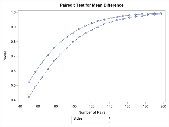
The “Computed Power” table in Output 71.3.1 shows that the power with 100 patients is about 0.8 for the two-sided test and 0.87 for the one-sided test with the alternative of larger Brantium mean. In Output 71.3.2, the line style identifies the number of sides of the test. The plotting symbols identify locations of actual computed powers; the curves are linear interpolations of these points. The plot demonstrates how much higher the power is in the one-sided test than in the two-sided test for the range of sample sizes.
Suppose now that instead of detecting a difference between Xilodol and Brantium, you want to establish that they are similar—in particular, that the absolute mean PEF difference is at most 35. You might consider this goal if, for example, one of the drugs has fewer side effects and if a difference of no more than 35 is considered clinically small. Instead of a standard t test, you would conduct an equivalence test of the treatment mean difference for the two drugs. You would test the hypothesis that the true difference is less than –35 or more than 35 against the alternative that the mean difference is between –35 and 35, by using an additive model and a two one-sided tests (“TOST”) analysis.
Assuming no period effect, you can use the PAIREDMEANS statement with the TEST=EQUIV_DIFF option to perform a sample size analysis for the paired equivalence test. Indicate power as the result parameter by specifying the POWER= option with a missing value (.). Use the LOWER= and UPPER= options to specify the equivalence bounds of –35 and 35. Use the PAIREDMEANS=, PAIREDSTDDEVS=, CORR=, and ALPHA= options in the same way as in the t test at the beginning of this example to specify the remaining parameters.
The following statements perform the sample size analysis:
proc power;
   pairedmeans test=equiv_add
      lower         = -35
      upper         = 35
      pairedmeans   = (330 310)
      pairedstddevs = (40 55)
      corr          = 0.3
      alpha         = 0.01
      npairs        = 100
      power         = .;
run;
The default option DIST=NORMAL specifies an assumption of normally distributed data. The output is shown in Output 71.3.3.
Output 71.3.3: Power for Paired Equivalence Test for Crossover Design
| Fixed Scenario Elements | |
|---|---|
| Distribution | Normal |
| Method | Exact |
| Lower Equivalence Bound | -35 |
| Upper Equivalence Bound | 35 |
| Alpha | 0.01 |
| Reference Mean | 330 |
| Treatment Mean | 310 |
| Standard Deviation 1 | 40 |
| Standard Deviation 2 | 55 |
| Correlation | 0.3 |
| Number of Pairs | 100 |
| Computed Power |
|---|
| Power |
| 0.598 |
The power for the paired equivalence test with 100 patients is about 0.6.