The POWER Procedure
- Overview
-
Getting Started

-
Syntax
-
Details
-
ExamplesOne-Way ANOVAThe Sawtooth Power Function in Proportion AnalysesSimple AB/BA Crossover DesignsNoninferiority Test with Lognormal DataMultiple Regression and CorrelationComparing Two Survival CurvesConfidence Interval PrecisionCustomizing PlotsBinary Logistic Regression with Independent PredictorsWilcoxon-Mann-Whitney Test
- References
This example deals with the same situation as in Example 44.1 of Chapter 44: The GLMPOWER Procedure.
Hocking (1985, p. 109) describes a study of the effectiveness of electrolytes in reducing lactic acid buildup for long-distance runners. You are planning a similar study in which you will allocate five different fluids to runners on a 10-mile course and measure lactic acid buildup immediately after the run. The fluids consist of water and two commercial electrolyte drinks, EZDure and LactoZap, each prepared at two concentrations, low (EZD1 and LZ1) and high (EZD2 and LZ2).
You conjecture that the standard deviation of lactic acid measurements given any particular fluid is about 3.75, and that the expected lactic acid values will correspond roughly to those in Table 71.32. You are least familiar with the LZ1 drink and hence decide to consider a range of reasonable values for that mean.
You are interested in four different comparisons, shown in Table 71.33 with appropriate contrast coefficients.
Table 71.33: Planned Comparisons
|
Contrast Coefficients |
|||||
|---|---|---|---|---|---|
|
Comparison |
Water |
EZD1 |
EZD2 |
LZ1 |
LZ2 |
|
Water versus electrolytes |
4 |
–1 |
–1 |
–1 |
–1 |
|
EZD versus LZ |
0 |
1 |
1 |
–1 |
–1 |
|
EZD1 versus EZD2 |
0 |
1 |
–1 |
0 |
0 |
|
LZ1 versus LZ2 |
0 |
0 |
0 |
1 |
–1 |
For each of these contrasts you want to determine the sample size required to achieve a power of 0.9 for detecting an effect
with magnitude in accord with Table 71.32. You are not yet attempting to choose a single sample size for the study, but rather checking the range of sample sizes needed
for individual contrasts. You plan to test each contrast at ![]() . In the interests of reducing costs, you will provide twice as many runners with water as with any of the electrolytes; in
other words, you will use a sample size weighting scheme of 2:1:1:1:1. Use the ONEWAYANOVA statement in the POWER procedure to compute the sample sizes.
. In the interests of reducing costs, you will provide twice as many runners with water as with any of the electrolytes; in
other words, you will use a sample size weighting scheme of 2:1:1:1:1. Use the ONEWAYANOVA statement in the POWER procedure to compute the sample sizes.
The statements required to perform this analysis are as follows:
proc power;
   onewayanova
      groupmeans = 35.6 | 33.7 | 30.2 | 29 28 | 25.9
      stddev = 3.75
      groupweights = (2 1 1 1 1)
      alpha = 0.025
      ntotal = .
      power = 0.9
      contrast = (4 -1 -1 -1 -1) (0  1  1 -1 -1)
                 (0  1 -1  0  0) (0  0  0  1 -1);
run;
The NTOTAL= option with a missing value (.) indicates total sample size as the result parameter. The GROUPMEANS= option with values from Table 71.32 specifies your conjectures for the means. With only one mean varying (the LZ1 mean), the “crossed” notation is simpler, showing scenarios for each group mean, separated by vertical bars (|). See the section Specifying Value Lists in Analysis Statements for more details on crossed and matched notations for grouped values. The contrasts in Table 71.33 are specified with the CONTRAST= option, by using the “matched” notation with each contrast enclosed in parentheses. The STDDEV=, ALPHA=, and POWER= options specify the error standard deviation, significance level, and power. The GROUPWEIGHTS= option specifies the weighting schemes. Default values for the NULLCONTRAST= and SIDES= options specify a two-sided t test of the contrast equal to 0. See Output 71.1.1 for the results.
Output 71.1.1: Sample Sizes for One-Way ANOVA Contrasts
| Fixed Scenario Elements | |
|---|---|
| Method | Exact |
| Alpha | 0.025 |
| Standard Deviation | 3.75 |
| Group Weights | 2 1 1 1 1 |
| Nominal Power | 0.9 |
| Number of Sides | 2 |
| Null Contrast Value | 0 |
| Computed N Total | ||||||||||||
|---|---|---|---|---|---|---|---|---|---|---|---|---|
| Index | Contrast | Means | Actual Power | N Total | ||||||||
| 1 | 4 | -1 | -1 | -1 | -1 | 35.6 | 33.7 | 30.2 | 29 | 25.9 | 0.947 | 30 |
| 2 | 4 | -1 | -1 | -1 | -1 | 35.6 | 33.7 | 30.2 | 28 | 25.9 | 0.901 | 24 |
| 3 | 0 | 1 | 1 | -1 | -1 | 35.6 | 33.7 | 30.2 | 29 | 25.9 | 0.929 | 60 |
| 4 | 0 | 1 | 1 | -1 | -1 | 35.6 | 33.7 | 30.2 | 28 | 25.9 | 0.922 | 48 |
| 5 | 0 | 1 | -1 | 0 | 0 | 35.6 | 33.7 | 30.2 | 29 | 25.9 | 0.901 | 174 |
| 6 | 0 | 1 | -1 | 0 | 0 | 35.6 | 33.7 | 30.2 | 28 | 25.9 | 0.901 | 174 |
| 7 | 0 | 0 | 0 | 1 | -1 | 35.6 | 33.7 | 30.2 | 29 | 25.9 | 0.902 | 222 |
| 8 | 0 | 0 | 0 | 1 | -1 | 35.6 | 33.7 | 30.2 | 28 | 25.9 | 0.902 | 480 |
The sample sizes in Output 71.1.1 range from 24 for the comparison of water versus electrolytes to 480 for the comparison of LZ1 versus LZ2, both assuming
the smaller LZ1 mean. The sample size for the latter comparison is relatively large because the small mean difference of ![]() is hard to detect.
is hard to detect.
The Nominal Power of 0.9 in the “Fixed Scenario Elements” table in Output 71.1.1 represents the input target power, and the Actual Power column in the “Computed N Total” table is the power at the sample size (N Total) adjusted to achieve the specified sample weighting. Note that all of the sample sizes are rounded up to multiples of 6 to preserve integer group sizes (since the group weights add up to 6). You can use the NFRACTIONAL option in the ONEWAYANOVA statement to compute raw fractional sample sizes.
Suppose you want to plot the required sample size for the range of power values from 0.5 to 0.95. First, define the analysis by specifying the same statements as before, but add the PLOTONLY option to the PROC POWER statement to disable the nongraphical results. Next, specify the PLOT statement with X=POWER to request a plot with power on the X axis. (The result parameter, here sample size, is always plotted on the other axis.) Use the MIN= and MAX= options in the PLOT statement to specify the power range. The following statements produce the plot shown in Output 71.1.2.
ods listing style=htmlbluecml;
ods graphics on;

proc power plotonly;
   onewayanova
      groupmeans = 35.6 | 33.7 | 30.2 | 29 28 | 25.9
      stddev = 3.75
      groupweights = (2 1 1 1 1)
      alpha = 0.025
      ntotal = .
      power = 0.9
      contrast = (4 -1 -1 -1 -1) (0  1  1 -1 -1)
                 (0  1 -1  0  0) (0  0  0  1 -1);
   plot x=power min=.5 max=.95;
run;
The ODS LISTING STYLE=HTMLBLUECML statement specifies the HTMLBLUECML style, which is suitable for use with PROC POWER because it allows both marker symbols and line styles to vary. See the section ODS Styles Suitable for Use with PROC POWER for more information.
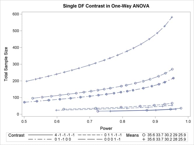
In Output 71.1.2, the line style identifies the contrast, and the plotting symbol identifies the group means scenario. The plot shows that the required sample size is highest for the (0 0 0 1 –1) contrast, corresponding to the test of LZ1 versus LZ2 that was previously found to require the most resources, in either cell means scenario.
Note that some of the plotted points in Output 71.1.2 are unevenly spaced. This is because the plotted points are the rounded sample size results at their corresponding actual power levels. The range specified with the MIN= and MAX= values in the PLOT statement corresponds to nominal power levels. In some cases, actual power is substantially higher than nominal power. To obtain plots with evenly spaced points (but with fractional sample sizes at the computed points), you can use the NFRACTIONAL option in the analysis statement preceding the PLOT statement.
Finally, suppose you want to plot the power for the range of sample sizes you will likely consider for the study (the range of 24 to 480 that achieves 0.9 power for different comparisons). In the ONEWAYANOVA statement, identify power as the result (POWER=.), and specify NTOTAL=24. The following statements produce the plot:
proc power plotonly;
   onewayanova
      groupmeans = 35.6 | 33.7 | 30.2 | 29 28 | 25.9
      stddev = 3.75
      groupweights = (2 1 1 1 1)
      alpha = 0.025
      ntotal = 24
      power = .
      contrast = (4 -1 -1 -1 -1) (0  1  1 -1 -1)
                 (0  1 -1  0  0) (0  0  0  1 -1);
   plot x=n min=24 max=480;
run;

ods graphics off;
The X=N option in the PLOT statement requests a plot with sample size on the X axis.
Note that the value specified with the NTOTAL=24 option is not used. It is overridden in the plot by the MIN= and MAX= options in the PLOT statement, and the PLOTONLY option in the PROC POWER statement disables nongraphical results. But the NTOTAL= option (along with a value) is still needed in the ONEWAYANOVA statement as a placeholder, to identify the desired parameterization for sample size.
Output 71.1.3 shows the resulting plot.
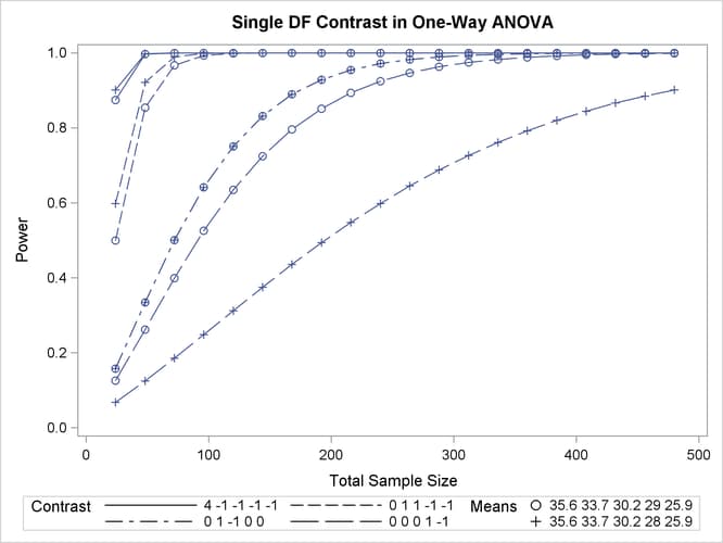
Although Output 71.1.2 and Output 71.1.3 surface essentially the same computations for practical power ranges, they each provide a different quick visual assessment. Output 71.1.2 reveals the range of required sample sizes for powers of interest, and Output 71.1.3 reveals the range of achieved powers for sample sizes of interest.