The POWER Procedure
- Overview
-
Getting Started

-
Syntax
-
Details
-
ExamplesOne-Way ANOVAThe Sawtooth Power Function in Proportion AnalysesSimple AB/BA Crossover DesignsNoninferiority Test with Lognormal DataMultiple Regression and CorrelationComparing Two Survival CurvesConfidence Interval PrecisionCustomizing PlotsBinary Logistic Regression with Independent PredictorsWilcoxon-Mann-Whitney Test
- References
The hypotheses for the two-sample t test are
|
|
|
|
|
 |
The test assumes normally distributed data and common standard deviation per group, and it requires ![]() ,
, ![]() , and
, and ![]() . The test statistics are
. The test statistics are
|
|
|
|
|
|
where ![]() and
and ![]() are the sample means and
are the sample means and ![]() is the pooled standard deviation, and
is the pooled standard deviation, and
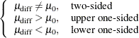
The test is
![\[ \mbox{Reject} \quad H_0 \quad \mbox{if} \left\{ \begin{array}{ll} t^2 \ge F_{1-\alpha }(1, N-2), & \mbox{two-sided} \\ t \ge t_{1-\alpha }(N-2), & \mbox{upper one-sided} \\ t \le t_{\alpha }(N-2), & \mbox{lower one-sided} \\ \end{array} \right. \]](images/statug_power0806.png)
Exact power computations for t tests are given in O’Brien and Muller (1993, Section 8.2.1):
|
|
 |
Solutions for N, ![]() ,
, ![]() ,
, ![]() , and
, and ![]() are obtained by numerically inverting the power equation. Closed-form solutions for other parameters, in terms of
are obtained by numerically inverting the power equation. Closed-form solutions for other parameters, in terms of ![]() , are as follows:
, are as follows:
|
|
|
|
|
|
|
|
|
|
|
|
|
|
|
|
|
|
Finally, here is a derivation of the solution for ![]() :
:
Solve the ![]() equation for
equation for ![]() (which requires the quadratic formula). Then determine the range of
(which requires the quadratic formula). Then determine the range of ![]() given
given ![]() :
:
|
|
|
|
|
|
This implies
The hypotheses for the two-sample Satterthwaite t test are
|
|
|
|
|
|
The test assumes normally distributed data and requires ![]() ,
, ![]() , and
, and ![]() . The test statistics are
. The test statistics are
|
|
![$\displaystyle = \frac{\bar{x}_2-\bar{x}_1-\mu _0}{\left[\frac{s_1^2}{n_1} + \frac{s_2^2}{n_2}\right]^\frac {1}{2}} = N^\frac {1}{2} \frac{\bar{x}_2-\bar{x}_1-\mu _0}{\left[\frac{s_1^2}{w_1} + \frac{s_2^2}{w_2}\right]^\frac {1}{2}} $](images/statug_power0828.png) |
|
|
|
where ![]() and
and ![]() are the sample means and
are the sample means and ![]() and
and ![]() are the sample standard deviations.
are the sample standard deviations.
DiSantostefano and Muller (1995, p. 585) state, the test is based on assuming that under ![]() , F is distributed as
, F is distributed as ![]() , where
, where ![]() is given by Satterthwaite’s approximation (Satterthwaite, 1946),
is given by Satterthwaite’s approximation (Satterthwaite, 1946),
![\[ \nu = \frac{\left[\frac{\sigma _1^2}{n_1} + \frac{\sigma _2^2}{n_2}\right]^2}{\frac{\left[\frac{\sigma _1^2}{n_1}\right]^2}{n_1-1} + \frac{\left[\frac{\sigma _2^2}{n_2}\right]^2}{n_2-1}} = \frac{\left[\frac{\sigma _1^2}{w_1} + \frac{\sigma _2^2}{w_2}\right]^2}{\frac{\left[\frac{\sigma _1^2}{w_1}\right]^2}{N w_1-1} + \frac{\left[\frac{\sigma _2^2}{w_2}\right]^2}{N w_2-1}} \]](images/statug_power0834.png)
Since ![]() is unknown, in practice it must be replaced by an estimate
is unknown, in practice it must be replaced by an estimate
![\[ \hat{\nu } = \frac{\left[\frac{s_1^2}{n_1} + \frac{s_2^2}{n_2}\right]^2}{\frac{\left[\frac{s_1^2}{n_1}\right]^2}{n_1-1} + \frac{\left[\frac{s_2^2}{n_2}\right]^2}{n_2-1}} = \frac{\left[\frac{s_1^2}{w_1} + \frac{s_2^2}{w_2}\right]^2}{\frac{\left[\frac{s_1^2}{w_1}\right]^2}{N w_1-1} + \frac{\left[\frac{s_2^2}{w_2}\right]^2}{N w_2-1}} \]](images/statug_power0835.png)
So the test is
![\[ \mbox{Reject} \quad H_0 \quad \mbox{if} \left\{ \begin{array}{ll} F \ge F_{1-\alpha }(1, \hat{\nu }), & \mbox{two-sided} \\ t \ge t_{1-\alpha }(\hat{\nu }), & \mbox{upper one-sided} \\ t \le t_{\alpha }(\hat{\nu }), & \mbox{lower one-sided} \\ \end{array} \right. \]](images/statug_power0836.png)
Exact solutions for power for the two-sided and upper one-sided cases are given in Moser, Stevens, and Watts (1989). The lower one-sided case follows easily by using symmetry. The equations are as follows:
|
|
![$\displaystyle = \left\{ \begin{array}{ll} \int _0^\infty P\left(F(1,N-2, \lambda ) > \right. \\ \quad \left. h(u) F_{1-\alpha }(1, v(u)) | u\right) f(u) \mr {d}u, & \mbox{two-sided} \\ \int _0^\infty P\left(t(N-2, \lambda ^\frac {1}{2}) > \right. \\ \quad \left. \left[h(u)\right]^\frac {1}{2} t_{1-\alpha }(v(u)) | u\right) f(u) \mr {d}u, & \mbox{upper one-sided} \\ \int _0^\infty P\left(t(N-2, \lambda ^\frac {1}{2}) < \right. \\ \quad \left. \left[h(u)\right]^\frac {1}{2} t_{\alpha }(v(u)) | u\right) f(u) \mr {d}u, & \mbox{lower one-sided} \\ \end{array} \right. $](images/statug_power0838.png) |
|
|
|
|
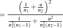
|
![$\displaystyle = \frac{\left(\frac{1}{n_1} + \frac{u}{n_2}\right) (n_1+n_2-2)}{\left[(n_1-1) + (n_2-1)\frac{u\sigma _1^2}{\sigma _2^2}\right] \left(\frac{1}{n_1} + \frac{\sigma _2^2}{\sigma _1^2n_2}\right)} $](images/statug_power0841.png) |
|
|
 |
|
|
|
|
|
![$\displaystyle = \frac{\Gamma \left(\frac{n_1+n_2-2}{2}\right)}{\Gamma \left(\frac{n_1-1}{2}\right) \Gamma \left(\frac{n_2-1}{2}\right)} \left[ \frac{\sigma _1^2(n_2-1)}{\sigma _2^2(n_1-1)}\right]^\frac {n_2-1}{2} u^\frac {n_2-3}{2} \left[1+\left(\frac{n_2-1}{n_1-1}\right) \frac{u\sigma _1^2}{\sigma _2^2}\right]^{-\left(\frac{n_1+n_2-2}{2}\right)} $](images/statug_power0847.png) |
The density ![]() is obtained from the fact that
is obtained from the fact that
The lognormal case is handled by reexpressing the analysis equivalently as a normality-based test on the log-transformed data, by using properties of the lognormal distribution as discussed in Johnson, Kotz, and Balakrishnan (1994, Chapter 14). The approaches in the section Two-Sample t Test Assuming Equal Variances (TEST=DIFF) then apply.
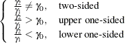
In contrast to the usual t test on normal data, the hypotheses with lognormal data are defined in terms of geometric means rather than arithmetic means. The test assumes equal coefficients of variation in the two groups.
The hypotheses for the two-sample t test with lognormal data are
|
|
|
|
|
 |
Let ![]() ,
, ![]() , and
, and ![]() be the (arithmetic) means and common standard deviation of the corresponding normal distributions of the log-transformed
data. The hypotheses can be rewritten as follows:
be the (arithmetic) means and common standard deviation of the corresponding normal distributions of the log-transformed
data. The hypotheses can be rewritten as follows:
|
|
|
|
|
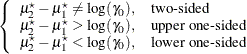 |
where
|
|
|
|
|
|
The test assumes lognormally distributed data and requires ![]() ,
, ![]() , and
, and ![]() .
.
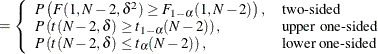
The power is
![\[ \mr {power} = \left\{ \begin{array}{ll} P\left(F(1, N-2, \delta ^2) \ge F_{1-\alpha }(1, N-2)\right), & \mbox{two-sided} \\ P\left(t(N-2, \delta ) \ge t_{1-\alpha }(N-2)\right), & \mbox{upper one-sided} \\ P\left(t(N-2, \delta ) \le t_{\alpha }(N-2)\right), & \mbox{lower one-sided} \\ \end{array} \right. \]](images/statug_power0851.png)
where
|
|
|
|
|
|
The hypotheses for the equivalence test are
|
|
|
|
|
|
The analysis is the two one-sided tests (TOST) procedure of Schuirmann (1987). The test assumes normally distributed data and requires ![]() ,
, ![]() , and
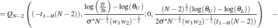
, and ![]() . Phillips (1990) derives an expression for the exact power assuming a balanced design; the results are easily adapted to an unbalanced design:
. Phillips (1990) derives an expression for the exact power assuming a balanced design; the results are easily adapted to an unbalanced design:
|
|
|
|
|
|
where ![]() is Owen’s Q function, defined in the section Common Notation.
is Owen’s Q function, defined in the section Common Notation.
The lognormal case is handled by reexpressing the analysis equivalently as a normality-based test on the log-transformed data, by using properties of the lognormal distribution as discussed in Johnson, Kotz, and Balakrishnan (1994, Chapter 14). The approaches in the section Additive Equivalence Test for Mean Difference with Normal Data (TEST=EQUIV_DIFF) then apply.
In contrast to the additive equivalence test on normal data, the hypotheses with lognormal data are defined in terms of geometric means rather than arithmetic means.
The hypotheses for the equivalence test are
|
|
|
|
|
|
The analysis is the two one-sided tests (TOST) procedure of Schuirmann (1987) on the log-transformed data. The test assumes lognormally distributed data and requires ![]() ,
, ![]() , and
, and ![]() . Diletti, Hauschke, and Steinijans (1991) derive an expression for the exact power assuming a crossover design; the results are easily adapted to an unbalanced two-sample
design:
. Diletti, Hauschke, and Steinijans (1991) derive an expression for the exact power assuming a crossover design; the results are easily adapted to an unbalanced two-sample
design:
|
|
 |
|
|
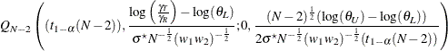 |
where
is the (assumed common) standard deviation of the normal distribution of the log-transformed data, and ![]() is Owen’s Q function, defined in the section Common Notation.
is Owen’s Q function, defined in the section Common Notation.
This analysis of precision applies to the standard t-based confidence interval:
![\[ \begin{array}{ll} \left[ (\bar{x}_2 - \bar{x}_1) - t_{1-\frac{\alpha }{2}}(N-2) \frac{s_ p}{\sqrt {N w_1 w_2}}, \right. \\ \quad \left. (\bar{x}_2 - \bar{x}_1) + t_{1-\frac{\alpha }{2}}(N-2) \frac{s_ p}{\sqrt {N w_1 w_2}} \right], & \mbox{two-sided} \\ \left[ (\bar{x}_2 - \bar{x}_1) - t_{1-\alpha }(N-2) \frac{s_ p}{\sqrt {N w_1 w_2}}, \quad \infty \right), & \mbox{upper one-sided} \\ \left( -\infty , \quad (\bar{x}_2 - \bar{x}_1) + t_{1-\alpha }(N-2) \frac{s_ p}{\sqrt {N w_1 w_2}} \right], & \mbox{lower one-sided} \\ \end{array} \]](images/statug_power0860.png)
where ![]() and
and ![]() are the sample means and
are the sample means and ![]() is the pooled standard deviation. The “half-width” is defined as the distance from the point estimate
is the pooled standard deviation. The “half-width” is defined as the distance from the point estimate ![]() to a finite endpoint,
to a finite endpoint,
A “valid” conference interval captures the true mean. The exact probability of obtaining at most the target confidence interval half-width h, unconditional or conditional on validity, is given by Beal (1989):
|
|
 |
|
|
![$\displaystyle = \left\{ \begin{array}{ll} \left(\frac{1}{1-\alpha }\right) 2 \left[ Q_{N-2}\left((t_{1-\frac{\alpha }{2}}(N-2)),0; \right. \right. \\ \quad \left. \left. 0,b_2\right) - Q_{N-2}(0,0;0,b_2)\right], & \mbox{two-sided} \\ \left(\frac{1}{1-\alpha }\right) Q_{N-2}\left((t_{1-\alpha }(N-2)),0;0,b_2\right), & \mbox{one-sided} \\ \end{array} \right. $](images/statug_power0865.png) |
where
|
|
|
|
|
|
and ![]() is Owen’s Q function, defined in the section Common Notation.
is Owen’s Q function, defined in the section Common Notation.
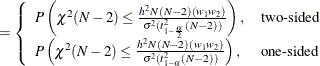
A “quality” confidence interval is both sufficiently narrow (half-width ![]() ) and valid:
) and valid:
|
|
|
|
|
|