The LOGISTIC Procedure
- Overview
- Getting Started
-
Syntax
 PROC LOGISTIC StatementBY StatementCLASS StatementCODE StatementCONTRAST StatementEFFECT StatementEFFECTPLOT StatementESTIMATE StatementEXACT StatementEXACTOPTIONS StatementFREQ StatementID StatementLSMEANS StatementLSMESTIMATE StatementMODEL StatementNLOPTIONS StatementODDSRATIO StatementOUTPUT StatementROC StatementROCCONTRAST StatementSCORE StatementSLICE StatementSTORE StatementSTRATA StatementTEST StatementUNITS StatementWEIGHT Statement
 -
DetailsMissing ValuesResponse Level OrderingLink Functions and the Corresponding DistributionsDetermining Observations for Likelihood ContributionsIterative Algorithms for Model FittingConvergence CriteriaExistence of Maximum Likelihood EstimatesEffect-Selection MethodsModel Fitting InformationGeneralized Coefficient of DeterminationScore Statistics and TestsConfidence Intervals for ParametersOdds Ratio EstimationRank Correlation of Observed Responses and Predicted ProbabilitiesLinear Predictor, Predicted Probability, and Confidence LimitsClassification TableOverdispersionThe Hosmer-Lemeshow Goodness-of-Fit TestReceiver Operating Characteristic CurvesTesting Linear Hypotheses about the Regression CoefficientsRegression DiagnosticsScoring Data SetsConditional Logistic RegressionExact Conditional Logistic RegressionInput and Output Data SetsComputational ResourcesDisplayed OutputODS Table NamesODS Graphics
-
ExamplesStepwise Logistic Regression and Predicted ValuesLogistic Modeling with Categorical PredictorsOrdinal Logistic RegressionNominal Response Data: Generalized Logits ModelStratified SamplingLogistic Regression DiagnosticsROC Curve, Customized Odds Ratios, Goodness-of-Fit Statistics, R-Square, and Confidence LimitsComparing Receiver Operating Characteristic CurvesGoodness-of-Fit Tests and SubpopulationsOverdispersionConditional Logistic Regression for Matched Pairs DataFirth’s Penalized Likelihood Compared with Other ApproachesComplementary Log-Log Model for Infection RatesComplementary Log-Log Model for Interval-Censored Survival TimesScoring Data SetsUsing the LSMEANS StatementPartial Proportional Odds Model
- References
This example plots an ROC curve, estimates a customized odds ratio, produces the traditional goodness-of-fit analysis, displays
the generalized R Square measures for the fitted model, calculates the normal confidence intervals for the regression parameters,
and produces a display of the probability function and prediction curves for the fitted model. The data consist of three variables:
n (number of subjects in the sample), disease (number of diseased subjects in the sample), and age (age for the sample). A linear logistic regression model is used to study the effect of age on the probability of contracting
the disease. The statements to produce the data set and perform the analysis are as follows:
data Data1;
   input disease n age;
   datalines;
 0 14 25
 0 20 35
 0 19 45
 7 18 55
 6 12 65
17 17 75
;
ods graphics on;
proc logistic data=Data1 plots(only)=roc(id=obs);
   model disease/n=age / scale=none
                         clparm=wald
                         clodds=pl
                         rsquare;
   units age=10;
   effectplot;
run;
ods graphics off;
The option SCALE=NONE is specified to produce the deviance and Pearson goodness-of-fit analysis without adjusting for overdispersion. The RSQUARE option is specified to produce generalized R Square measures of the fitted model. The CLPARM=WALD option is specified to produce the Wald confidence intervals for the regression parameters. The UNITS statement is specified to produce customized odds ratio estimates for a change of 10 years in the age variable, and the CLODDS=PL option is specified to produce profile-likelihood confidence limits for the odds ratio. The PLOTS= option with ODS Graphics enabled produces a graphical display of the ROC curve, and the EFFECTPLOT statement displays the model fit.
The results in Output 54.7.1 show that the deviance and Pearson statistics indicate no lack of fit in the model.
Output 54.7.1: Deviance and Pearson Goodness-of-Fit Analysis
| Deviance and Pearson Goodness-of-Fit Statistics | ||||
|---|---|---|---|---|
| Criterion | Value | DF | Value/DF | Pr > ChiSq |
| Deviance | 7.7756 | 4 | 1.9439 | 0.1002 |
| Pearson | 6.6020 | 4 | 1.6505 | 0.1585 |
Output 54.7.2 shows that the R-square for the model is 0.74. The odds of an event increases by a factor of 7.9 for each 10-year increase in age.
Output 54.7.2: R-Square, Confidence Intervals, and Customized Odds Ratio
| Model Fit Statistics | |||
|---|---|---|---|
| Criterion | Intercept Only | Intercept and Covariates | |
| Log Likelihood | Full Log Likelihood | ||
| AIC | 124.173 | 52.468 | 18.075 |
| SC | 126.778 | 57.678 | 23.285 |
| -2 Log L | 122.173 | 48.468 | 14.075 |
| R-Square | 0.5215 | Max-rescaled R-Square | 0.8925 |
|---|
| Testing Global Null Hypothesis: BETA=0 | |||
|---|---|---|---|
| Test | Chi-Square | DF | Pr > ChiSq |
| Likelihood Ratio | 73.7048 | 1 | <.0001 |
| Score | 55.3274 | 1 | <.0001 |
| Wald | 23.3475 | 1 | <.0001 |
| Analysis of Maximum Likelihood Estimates | |||||
|---|---|---|---|---|---|
| Parameter | DF | Estimate | Standard Error |
Wald Chi-Square |
Pr > ChiSq |
| Intercept | 1 | -12.5016 | 2.5555 | 23.9317 | <.0001 |
| age | 1 | 0.2066 | 0.0428 | 23.3475 | <.0001 |
| Association of Predicted Probabilities and Observed Responses |
|||
|---|---|---|---|
| Percent Concordant | 92.6 | Somers' D | 0.906 |
| Percent Discordant | 2.0 | Gamma | 0.958 |
| Percent Tied | 5.4 | Tau-a | 0.384 |
| Pairs | 2100 | c | 0.953 |
| Parameter Estimates and Wald Confidence Intervals |
|||
|---|---|---|---|
| Parameter | Estimate | 95% Confidence Limits | |
| Intercept | -12.5016 | -17.5104 | -7.4929 |
| age | 0.2066 | 0.1228 | 0.2904 |
| Odds Ratio Estimates and Profile-Likelihood Confidence Intervals |
||||
|---|---|---|---|---|
| Effect | Unit | Estimate | 95% Confidence Limits | |
| age | 10.0000 | 7.892 | 3.881 | 21.406 |
Since ODS Graphics is enabled, a graphical display of the ROC curve is produced as shown in Output 54.7.3.
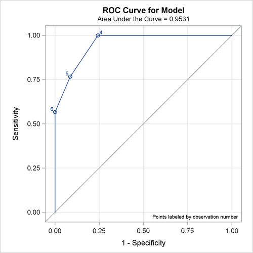
Note that the area under the ROC curve is estimated by the statistic c in the “Association of Predicted Probabilities and Observed Responses” table. In this example, the area under the ROC curve is 0.953.
Since there is only one continuous covariate and since ODS Graphics is enabled, the EFFECTPLOT statement produces a graphical display of the predicted probability curve with bounding 95% confidence limits as shown in Output 54.7.4.
