The LOGISTIC Procedure
- Overview
- Getting Started
-
Syntax
 PROC LOGISTIC StatementBY StatementCLASS StatementCODE StatementCONTRAST StatementEFFECT StatementEFFECTPLOT StatementESTIMATE StatementEXACT StatementEXACTOPTIONS StatementFREQ StatementID StatementLSMEANS StatementLSMESTIMATE StatementMODEL StatementNLOPTIONS StatementODDSRATIO StatementOUTPUT StatementROC StatementROCCONTRAST StatementSCORE StatementSLICE StatementSTORE StatementSTRATA StatementTEST StatementUNITS StatementWEIGHT Statement
 -
DetailsMissing ValuesResponse Level OrderingLink Functions and the Corresponding DistributionsDetermining Observations for Likelihood ContributionsIterative Algorithms for Model FittingConvergence CriteriaExistence of Maximum Likelihood EstimatesEffect-Selection MethodsModel Fitting InformationGeneralized Coefficient of DeterminationScore Statistics and TestsConfidence Intervals for ParametersOdds Ratio EstimationRank Correlation of Observed Responses and Predicted ProbabilitiesLinear Predictor, Predicted Probability, and Confidence LimitsClassification TableOverdispersionThe Hosmer-Lemeshow Goodness-of-Fit TestReceiver Operating Characteristic CurvesTesting Linear Hypotheses about the Regression CoefficientsRegression DiagnosticsScoring Data SetsConditional Logistic RegressionExact Conditional Logistic RegressionInput and Output Data SetsComputational ResourcesDisplayed OutputODS Table NamesODS Graphics
-
ExamplesStepwise Logistic Regression and Predicted ValuesLogistic Modeling with Categorical PredictorsOrdinal Logistic RegressionNominal Response Data: Generalized Logits ModelStratified SamplingLogistic Regression DiagnosticsROC Curve, Customized Odds Ratios, Goodness-of-Fit Statistics, R-Square, and Confidence LimitsComparing Receiver Operating Characteristic CurvesGoodness-of-Fit Tests and SubpopulationsOverdispersionConditional Logistic Regression for Matched Pairs DataFirth’s Penalized Likelihood Compared with Other ApproachesComplementary Log-Log Model for Infection RatesComplementary Log-Log Model for Interval-Censored Survival TimesScoring Data SetsUsing the LSMEANS StatementPartial Proportional Odds Model
- References
Scoring a data set, which is especially important for predictive modeling, means applying a previously fitted model to a new data set in order to compute the conditional, or posterior, probabilities of each response category given the values of the explanatory variables in each observation.
The SCORE statement enables you to score new data sets and output the scored values and, optionally, the corresponding confidence limits into a SAS data set. If the response variable is included in the new data set, then you can request fit statistics for the data, which is especially useful for test or validation data. If the response is binary, you can also create a SAS data set containing the receiver operating characteristic (ROC) curve. You can specify multiple SCORE statements in the same invocation of PROC LOGISTIC.
By default, the posterior probabilities are based on implicit prior probabilities that are proportional to the frequencies of the response categories in the training data (the data used to fit the model). Explicit prior probabilities should be specified with the PRIOR= or PRIOREVENT= option when the sample proportions of the response categories in the training data differ substantially from the operational data to be scored. For example, to detect a rare category, it is common practice to use a training set in which the rare categories are overrepresented; without prior probabilities that reflect the true incidence rate, the predicted posterior probabilities for the rare category will be too high. By specifying the correct priors, the posterior probabilities are adjusted appropriately.
The model fit to the DATA= data set in the PROC LOGISTIC statement is the default model used for the scoring. Alternatively, you can save a model fit in one run of PROC LOGISTIC and use it to score new data in a subsequent run. The OUTMODEL= option in the PROC LOGISTIC statement saves the model information in a SAS data set. Specifying this data set in the INMODEL= option of a new PROC LOGISTIC run will score the DATA= data set in the SCORE statement without refitting the model.
The STORE statement can also be used to save your model. The PLM procedure can use this model to score new data sets; see Chapter 69: The PLM Procedure, for more information. You cannot specify priors in PROC PLM.
Specifying the FITSTAT option displays the following fit statistics when the data set being scored includes the response variable:
|
Statistic |
Description |
|---|---|
|
Total frequency |
|
|
Total weight |
|
|
Log likelihood |
|
|
Full log likelihood |
|
|
Misclassification (error) rate |
|
|
AIC |
|
|
AICC |
|
|
BIC |
|
|
SC |
|
|
R-square |
|
|
Maximum-rescaled R-square |
|
|
AUC |
Area under the ROC curve |
|
Brier score (polytomous response) |
|
|
Brier score (binary response) |
|
|
Brier reliability (events/trials syntax) |
|
In the preceding table, ![]() is the frequency of the ith observation in the data set being scored,
is the frequency of the ith observation in the data set being scored, ![]() is the weight of the observation, and
is the weight of the observation, and ![]() . The number of trials when events/trials syntax is specified is
. The number of trials when events/trials syntax is specified is ![]() , and with single-trial syntax
, and with single-trial syntax ![]() . The values
. The values ![]() and
and ![]() are described in the section OUT= Output Data Set in a SCORE Statement. The indicator function
are described in the section OUT= Output Data Set in a SCORE Statement. The indicator function ![]() is 1 if A is true and 0 otherwise. The likelihood of the model is L, and
is 1 if A is true and 0 otherwise. The likelihood of the model is L, and ![]() denotes the likelihood of the intercept-only model. For polytomous response models,
denotes the likelihood of the intercept-only model. For polytomous response models, ![]() is the observed polytomous response level,
is the observed polytomous response level, ![]() is the predicted probability of the jth response level for observation i, and
is the predicted probability of the jth response level for observation i, and ![]() . For binary response models,
. For binary response models, ![]() is the predicted probability of the observation,
is the predicted probability of the observation, ![]() is the number of events when you specify events/trials syntax, and
is the number of events when you specify events/trials syntax, and ![]() when you specify single-trial syntax.
when you specify single-trial syntax.
The log likelihood, Akaike’s information criterion (AIC), and Schwarz criterion (SC) are described in the section Model Fitting Information. The full log likelihood is displayed for models specified with events/trials syntax, and the constant term is described in the section Model Fitting Information. The AICC is a small-sample bias-corrected version of the AIC (Hurvich and Tsai, 1993; Burnham and Anderson, 1998). The Bayesian information criterion (BIC) is the same as the SC except when events/trials syntax is specified. The area under the ROC curve for binary response models is defined in the section ROC Computations. The R-square and maximum-rescaled R-square statistics, defined in Generalized Coefficient of Determination, are not computed when you specify both an OFFSET= variable and the INMODEL= data set. The Brier score (Brier, 1950) is the weighted squared difference between the predicted probabilities and their observed response levels. For events/trials syntax, the Brier reliability is the weighted squared difference between the predicted probabilities and the observed proportions (Murphy, 1973).
Let F be the inverse link function. That is,
|
|
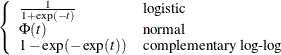 |
The first derivative of F is given by
|
|
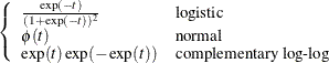 |
Suppose there are ![]() response categories. Let
response categories. Let Y be the response variable with levels ![]() . Let
. Let ![]() be a
be a ![]() -vector of covariates, with
-vector of covariates, with ![]() . Let
. Let ![]() be the vector of intercept and slope regression parameters.
be the vector of intercept and slope regression parameters.
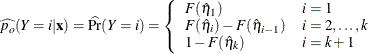
Posterior probabilities are given by
![\[ p(Y=i|\mb {x}) = \frac{p_ o(Y=i|\mb {x}) \frac{\widetilde{p}(Y=i)}{p_ o(Y=i)}}{\sum _ j p_ o(Y=j|\mb {x})\frac{\widetilde{p}(Y=j)}{p_ o(Y=j)}} \quad i=1,\ldots ,k+1 \]](images/statug_logistic0625.png)
where the old posterior probabilities (![]() ) are the conditional probabilities of the response categories given
) are the conditional probabilities of the response categories given ![]() , the old priors (
, the old priors (![]() ) are the sample proportions of response categories of the training data, and the new priors (
) are the sample proportions of response categories of the training data, and the new priors (![]() ) are specified in the PRIOR= or PRIOREVENT= option. To simplify notation, absorb the old priors into the new priors; that is
) are specified in the PRIOR= or PRIOREVENT= option. To simplify notation, absorb the old priors into the new priors; that is
Note if the PRIOR= and PRIOREVENT= options are not specified, then ![]() .
.
The posterior probabilities are functions of ![]() and their estimates are obtained by substituting
and their estimates are obtained by substituting ![]() by its MLE
by its MLE ![]() . The variances of the estimated posterior probabilities are given by the delta method as follows:
. The variances of the estimated posterior probabilities are given by the delta method as follows:
where
and the old posterior probabilities ![]() are described in the following sections.
are described in the following sections.
A 100(![]() )% confidence interval for
)% confidence interval for ![]() is
is
where ![]() is the upper 100
is the upper 100![]() percentile of the standard normal distribution.
percentile of the standard normal distribution.
Let ![]() be the intercept parameters and let
be the intercept parameters and let ![]() be the vector of slope parameters. Denote
be the vector of slope parameters. Denote ![]() . Let
. Let
Estimates of ![]() are obtained by substituting the maximum likelihood estimate
are obtained by substituting the maximum likelihood estimate ![]() for
for ![]() .
.
The predicted probabilities of the responses are
 |
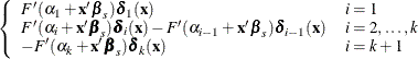
For ![]() , let
, let ![]() be a (k + 1) column vector with ith entry equal to 1, k + 1 entry equal to
be a (k + 1) column vector with ith entry equal to 1, k + 1 entry equal to ![]() , and all other entries 0. The derivative of
, and all other entries 0. The derivative of ![]() with respect to
with respect to ![]() are
are
|
|
 |
The cumulative posterior probabilities are
Their derivatives are
In the delta-method equation for the variance, replace ![]() with
with ![]() .
.
Finally, for the cumulative response model, use
|
|
|
|
|
|
|
|
|
|
|
|
|
|
|
|
Consider the last response level (Y=k+1) as the reference. Let ![]() be the (intercept and slope) parameter vectors for the first k logits, respectively. Denote
be the (intercept and slope) parameter vectors for the first k logits, respectively. Denote ![]() . Let
. Let ![]() with
with
Estimates of ![]() are obtained by substituting the maximum likelihood estimate
are obtained by substituting the maximum likelihood estimate ![]() for
for ![]() .
.
The predicted probabilities are
|
|
|
|
|
|
|
|
The derivative of ![]() with respect to
with respect to ![]() are
are
|
|
|
|
|
|
|
|
where
|
|
Let ![]() be the vector of regression parameters. Let
be the vector of regression parameters. Let
The variance of ![]() is given by
is given by
A 100(![]() ) percent confidence interval for
) percent confidence interval for ![]() is
is
Estimates of ![]() and confidence intervals for the
and confidence intervals for the ![]() are obtained by back-transforming
are obtained by back-transforming ![]() and the confidence intervals for
and the confidence intervals for ![]() , respectively. That is,
, respectively. That is,
and the confidence intervals are