The GENMOD Procedure
-
Overview

-
Getting Started
-
SyntaxPROC GENMOD StatementASSESS StatementBAYES StatementBY StatementCLASS StatementCODE StatementCONTRAST StatementDEVIANCE StatementEFFECTPLOT StatementESTIMATE StatementEXACT StatementEXACTOPTIONS StatementFREQ StatementFWDLINK StatementINVLINK StatementLSMEANS StatementLSMESTIMATE StatementMODEL StatementOUTPUT StatementProgramming StatementsREPEATED StatementSLICE StatementSTORE StatementSTRATA StatementVARIANCE StatementWEIGHT StatementZEROMODEL Statement
-
DetailsGeneralized Linear Models TheorySpecification of EffectsParameterization Used in PROC GENMODType 1 AnalysisType 3 AnalysisConfidence Intervals for ParametersF StatisticsLagrange Multiplier StatisticsPredicted Values of the MeanResidualsMultinomial ModelsZero-Inflated ModelsGeneralized Estimating EquationsAssessment of Models Based on Aggregates of ResidualsCase Deletion Diagnostic StatisticsBayesian AnalysisExact Logistic and Exact Poisson RegressionMissing ValuesDisplayed Output for Classical AnalysisDisplayed Output for Bayesian AnalysisDisplayed Output for Exact AnalysisODS Table NamesODS Graphics
-
ExamplesLogistic RegressionNormal Regression, Log Link Gamma Distribution Applied to Life DataOrdinal Model for Multinomial DataGEE for Binary Data with Logit Link FunctionLog Odds Ratios and the ALR AlgorithmLog-Linear Model for Count DataModel Assessment of Multiple Regression Using Aggregates of ResidualsAssessment of a Marginal Model for Dependent DataBayesian Analysis of a Poisson Regression ModelExact Poisson Regression
- References
This example illustrates the use of cumulative residuals to assess the adequacy of a marginal model for dependent data fit by generalized estimating equations (GEEs). The assessment methods are applied to CD4 count data from an AIDS clinical trial reported by Fischl, Richman, and Hansen (1990) and reanalyzed by Lin, Wei, and Ying (2002). The study randomly assigned 360 HIV patients to the drug AZT and 351 patients to placebo. CD4 counts were measured repeatedly over the course of the study. The data used here are the 4328 measurements taken in the first 40 weeks of the study.
The analysis focuses on the time trend of the response. The first model considered is
where ![]() is the time (in weeks) of the kth measurement on the ith patient,
is the time (in weeks) of the kth measurement on the ith patient, ![]() is the CD4 count at
is the CD4 count at ![]() for the ith patient, and
for the ith patient, and ![]() is the indicator of AZT for the ith patient. Normal errors and an independent working correlation are assumed.
is the indicator of AZT for the ith patient. Normal errors and an independent working correlation are assumed.
The following statements create the SAS data set cd4:
data cd4;
   input Id Y Time Time2 TrtTime TrtTime2;
   Time3 = Time2 * Time;
   TrtTime3 = TrtTime2 * Time;
   datalines;
1     264.00024       -0.28571        0.08163       -0.28571        0.08163
1     175.00070        4.14286       17.16327        4.14286       17.16327
1     306.00150        8.14286       66.30612        8.14286       66.30612
1     331.99835       12.14286      147.44898       12.14286      147.44898
1     309.99929       16.14286      260.59184       16.14286      260.59184
1     185.00077       28.71429      824.51020       28.71429      824.51020
1     175.00070       40.14286     1611.44898       40.14286     1611.44898
2     574.99998       -0.57143        0.32653        0.00000        0.00000

   ... more lines ...

711     363.99859        8.14286       66.30612        8.14286       66.30612
711     488.00224       12.14286      147.44898       12.14286      147.44898
711     240.00026       18.14286      329.16327       18.14286      329.16327
;
The following SAS statements fit the preceding model, create the cumulative residual plot in Output 40.9.1, and compute a p-value for the model.
To request these graphs, ODS Graphics must be enabled and you must specify the ASSESS statement. For general information about ODS Graphics, see Chapter 21: Statistical Graphics Using ODS. For specific information about the graphics available in the GENMOD procedure, see the section ODS Graphics.
Here, the SAS data set variables Time, Time2, TrtTime, and TrtTime2 correspond to ![]() ,
, ![]() ,
, ![]() , and
, and ![]() , respectively. The variable
, respectively. The variable Id identifies individual patients.
ods graphics on;

proc genmod data=cd4;
   class Id;
   model Y = Time Time2 TrtTime TrtTime2;
   repeated sub=Id;
   assess var=(Time) / resample
                       seed=603708000;
run;
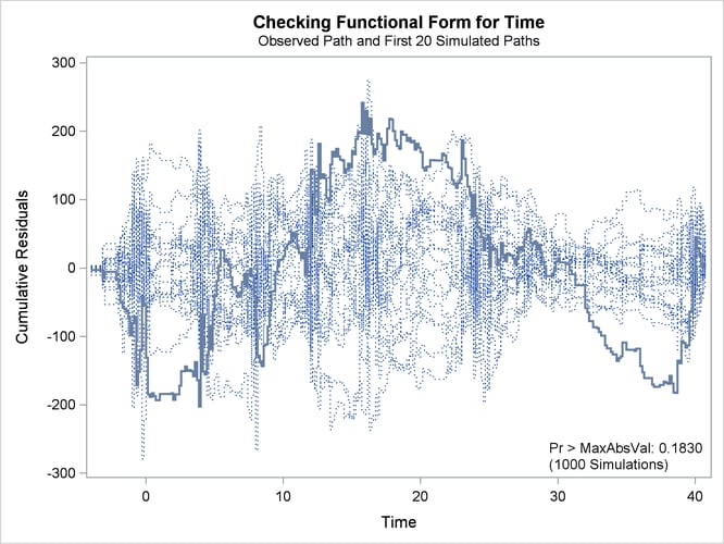
The cumulative residual plot in Output 40.9.1 displays cumulative residuals versus time for the model and 20 simulated realizations. The associated p-value, also shown in Output 40.9.1, is 0.18. These results indicate that a more satisfactory model might be possible. The observed cumulative residual pattern most resembles plot (c) in Output 40.8.6, suggesting cubic time trends.
The following SAS statements fit the model, create the plot in Output 40.9.2, and compute a p-value for a model with the additional terms ![]() and
and ![]() :
:
proc genmod data=cd4;
   class Id;
   model Y = Time Time2 Time3 TrtTime TrtTime2 TrtTime3;
   repeated sub=Id;
   assess var=(Time) / resample
                       seed=603708000;
run;
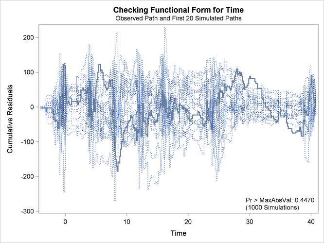
The observed cumulative residual pattern appears more typical of the simulated realizations, and the p-value is 0.45, indicating that the model with cubic time trends is more appropriate.