The GENMOD Procedure
-
Overview

-
Getting Started
-
SyntaxPROC GENMOD StatementASSESS StatementBAYES StatementBY StatementCLASS StatementCODE StatementCONTRAST StatementDEVIANCE StatementEFFECTPLOT StatementESTIMATE StatementEXACT StatementEXACTOPTIONS StatementFREQ StatementFWDLINK StatementINVLINK StatementLSMEANS StatementLSMESTIMATE StatementMODEL StatementOUTPUT StatementProgramming StatementsREPEATED StatementSLICE StatementSTORE StatementSTRATA StatementVARIANCE StatementWEIGHT StatementZEROMODEL Statement
-
DetailsGeneralized Linear Models TheorySpecification of EffectsParameterization Used in PROC GENMODType 1 AnalysisType 3 AnalysisConfidence Intervals for ParametersF StatisticsLagrange Multiplier StatisticsPredicted Values of the MeanResidualsMultinomial ModelsZero-Inflated ModelsGeneralized Estimating EquationsAssessment of Models Based on Aggregates of ResidualsCase Deletion Diagnostic StatisticsBayesian AnalysisExact Logistic and Exact Poisson RegressionMissing ValuesDisplayed Output for Classical AnalysisDisplayed Output for Bayesian AnalysisDisplayed Output for Exact AnalysisODS Table NamesODS Graphics
-
ExamplesLogistic RegressionNormal Regression, Log Link Gamma Distribution Applied to Life DataOrdinal Model for Multinomial DataGEE for Binary Data with Logit Link FunctionLog Odds Ratios and the ALR AlgorithmLog-Linear Model for Count DataModel Assessment of Multiple Regression Using Aggregates of ResidualsAssessment of a Marginal Model for Dependent DataBayesian Analysis of a Poisson Regression ModelExact Poisson Regression
- References
In this example the data, from Thall and Vail (1990), concern the treatment of people suffering from epileptic seizure episodes. These data are also analyzed in Diggle, Liang, and Zeger (1994). The data consist of the number of epileptic seizures in an eight-week baseline period, before any treatment, and in each of four two-week treatment periods, in which patients received either a placebo or the drug Progabide in addition to other therapy. A portion of the data is displayed in Table 40.16. See “Gee Model for Count Data, Exchangeable Correlation” in the SAS/STAT Sample Program Library for the complete data set.
Table 40.16: Epileptic Seizure Data
|
Patient ID |
Treatment |
Baseline |
Visit1 |
Visit2 |
Visit3 |
Visit4 |
|---|---|---|---|---|---|---|
|
104 |
Placebo |
11 |
5 |
3 |
3 |
3 |
|
106 |
Placebo |
11 |
3 |
5 |
3 |
3 |
|
107 |
Placebo |
6 |
2 |
4 |
0 |
5 |
|
. |
||||||
|
. |
||||||
|
. |
||||||
|
101 |
Progabide |
76 |
11 |
14 |
9 |
8 |
|
102 |
Progabide |
38 |
8 |
7 |
9 |
4 |
|
103 |
Progabide |
19 |
0 |
4 |
3 |
0 |
|
. |
||||||
|
. |
||||||
|
. |
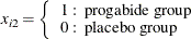
Model the data as a log-linear model with ![]() (the Poisson variance function) and
(the Poisson variance function) and
where
-
 number of epileptic seizures in interval j
-
 length of interval j
-
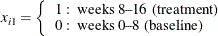
-
The correlations between the counts are modeled as ![]() ,
, ![]() (exchangeable correlations). For comparison, the correlations are also modeled as independent (identity correlation matrix).
In this model, the regression parameters have the interpretation in terms of the log seizure rate displayed in Table 40.17.
(exchangeable correlations). For comparison, the correlations are also modeled as independent (identity correlation matrix).
In this model, the regression parameters have the interpretation in terms of the log seizure rate displayed in Table 40.17.
Table 40.17: Interpretation of Regression Parameters
|
Treatment |
Visit |
|
|---|---|---|
|
Placebo |
Baseline |
|
|
1–4 |
|
|
|
Progabide |
Baseline |
|
|
1–4 |
|
The difference between the log seizure rates in the pretreatment (baseline) period and the treatment periods is ![]() for the placebo group and
for the placebo group and ![]() for the Progabide group. A value of
for the Progabide group. A value of ![]() indicates a reduction in the seizure rate.
indicates a reduction in the seizure rate.
Output 40.7.1 lists the first 14 observations of the data, which are arranged as one visit per observation:
Output 40.7.1: Partial Listing of the Seizure Data
| Obs | id | y | visit | trt | bline | age |
|---|---|---|---|---|---|---|
| 1 | 104 | 5 | 1 | 0 | 11 | 31 |
| 2 | 104 | 3 | 2 | 0 | 11 | 31 |
| 3 | 104 | 3 | 3 | 0 | 11 | 31 |
| 4 | 104 | 3 | 4 | 0 | 11 | 31 |
| 5 | 106 | 3 | 1 | 0 | 11 | 30 |
| 6 | 106 | 5 | 2 | 0 | 11 | 30 |
| 7 | 106 | 3 | 3 | 0 | 11 | 30 |
| 8 | 106 | 3 | 4 | 0 | 11 | 30 |
| 9 | 107 | 2 | 1 | 0 | 6 | 25 |
| 10 | 107 | 4 | 2 | 0 | 6 | 25 |
| 11 | 107 | 0 | 3 | 0 | 6 | 25 |
| 12 | 107 | 5 | 4 | 0 | 6 | 25 |
| 13 | 114 | 4 | 1 | 0 | 8 | 36 |
| 14 | 114 | 4 | 2 | 0 | 8 | 36 |
Some further data manipulations create an observation for the baseline measures, a log time interval variable for use as an offset, and an indicator variable for whether the observation is for a baseline measurement or a visit measurement. Patient 207 is deleted as an outlier, as in the Diggle, Liang, and Zeger (1994) analysis. The following statements prepare the data for analysis with PROC GENMOD:
data new;
   set thall;
   output;
   if visit=1 then do;
      y=bline;
      visit=0;
      output;
   end;
run;

data new;
   set new;
   if id ne 207;
   if visit=0 then do;
      x1=0;
      ltime=log(8);
   end;
   else do;
      x1=1;
      ltime=log(2);
   end;
run;
For comparison with the GEE results, an ordinary Poisson regression is first fit. The results are shown in Output 40.7.2.
Output 40.7.2: Maximum Likelihood Estimates
| Analysis Of Maximum Likelihood Parameter Estimates | |||||||
|---|---|---|---|---|---|---|---|
| Parameter | DF | Estimate | Standard Error | Wald 95% Confidence Limits | Wald Chi-Square | Pr > ChiSq | |
| Intercept | 1 | 1.3476 | 0.0341 | 1.2809 | 1.4144 | 1565.44 | <.0001 |
| x1 | 1 | 0.1108 | 0.0469 | 0.0189 | 0.2027 | 5.58 | 0.0181 |
| trt | 1 | -0.1080 | 0.0486 | -0.2034 | -0.0127 | 4.93 | 0.0264 |
| x1*trt | 1 | -0.3016 | 0.0697 | -0.4383 | -0.1649 | 18.70 | <.0001 |
| Scale | 0 | 1.0000 | 0.0000 | 1.0000 | 1.0000 | ||
| Note: | The scale parameter was held fixed. |
The GEE solution is requested with the REPEATED statement in the GENMOD procedure. The SUBJECT=ID option indicates that the
variable id describes the observations for a single cluster, and the CORRW option displays the working correlation matrix. The TYPE=
option specifies the correlation structure; the value EXCH indicates the exchangeable structure.
The following statements perform the analysis:
proc genmod data=new;
   class id;
   model y=x1 | trt / d=poisson offset=ltime;
   repeated subject=id / corrw covb type=exch;
run;
These statements first fit a generalized linear model (GLM) to these data by maximum likelihood. The estimates are not shown in the output, but are used as initial values for the GEE solution.
Information about the GEE model is displayed in Output 40.7.3. The results of fitting the model are displayed in Output 40.7.4. Compare these with the model of independence displayed in Output 40.7.2. The parameter estimates are nearly identical, but the standard errors for the independence case are underestimated. The
coefficient of the interaction term, ![]() , is highly significant under the independence model and marginally significant with the exchangeable correlations model.
, is highly significant under the independence model and marginally significant with the exchangeable correlations model.
Output 40.7.3: GEE Model Information
| GEE Model Information | |
|---|---|
| Correlation Structure | Exchangeable |
| Subject Effect | id (58 levels) |
| Number of Clusters | 58 |
| Correlation Matrix Dimension | 5 |
| Maximum Cluster Size | 5 |
| Minimum Cluster Size | 5 |
Output 40.7.4: GEE Parameter Estimates
| Analysis Of GEE Parameter Estimates | ||||||
|---|---|---|---|---|---|---|
| Empirical Standard Error Estimates | ||||||
| Parameter | Estimate | Standard Error | 95% Confidence Limits | Z | Pr > |Z| | |
| Intercept | 1.3476 | 0.1574 | 1.0392 | 1.6560 | 8.56 | <.0001 |
| x1 | 0.1108 | 0.1161 | -0.1168 | 0.3383 | 0.95 | 0.3399 |
| trt | -0.1080 | 0.1937 | -0.4876 | 0.2716 | -0.56 | 0.5770 |
| x1*trt | -0.3016 | 0.1712 | -0.6371 | 0.0339 | -1.76 | 0.0781 |
Table 40.18 displays the regression coefficients, standard errors, and normalized coefficients that result from fitting the model with independent and exchangeable working correlation matrices.
Table 40.18: Results of Model Fitting
|
Variable |
Correlation Structure |
Coef. |
Std. Error |
Coef./S.E. |
|---|---|---|---|---|
|
Intercept |
Exchangeable |
1.35 |
0.16 |
8.56 |
|
Independent |
1.35 |
0.03 |
39.52 |
|
|
Visit |
Exchangeable |
0.11 |
0.12 |
0.95 |
|
Independent |
0.11 |
0.05 |
2.36 |
|
|
Treat |
Exchangeable |
–0.11 |
0.19 |
–0.56 |
|
Independent |
–0.11 |
0.05 |
–2.22 |
|
|
|
Exchangeable |
–0.30 |
0.17 |
–1.76 |
|
Independent |
–0.30 |
0.07 |
–4.32 |
The fitted exchangeable correlation matrix is specified with the CORRW option and is displayed in Output 40.7.5.
Output 40.7.5: Working Correlation Matrix
| Working Correlation Matrix | |||||
|---|---|---|---|---|---|
| Col1 | Col2 | Col3 | Col4 | Col5 | |
| Row1 | 1.0000 | 0.5941 | 0.5941 | 0.5941 | 0.5941 |
| Row2 | 0.5941 | 1.0000 | 0.5941 | 0.5941 | 0.5941 |
| Row3 | 0.5941 | 0.5941 | 1.0000 | 0.5941 | 0.5941 |
| Row4 | 0.5941 | 0.5941 | 0.5941 | 1.0000 | 0.5941 |
| Row5 | 0.5941 | 0.5941 | 0.5941 | 0.5941 | 1.0000 |
If you specify the COVB option, you produce both the model-based (naive) and the empirical (robust) covariance matrices. Output 40.7.6 contains these estimates.
Output 40.7.6: Covariance Matrices
| Covariance Matrix (Model-Based) | ||||
|---|---|---|---|---|
| Prm1 | Prm2 | Prm3 | Prm4 | |
| Prm1 | 0.01223 | 0.001520 | -0.01223 | -0.001520 |
| Prm2 | 0.001520 | 0.01519 | -0.001520 | -0.01519 |
| Prm3 | -0.01223 | -0.001520 | 0.02495 | 0.005427 |
| Prm4 | -0.001520 | -0.01519 | 0.005427 | 0.03748 |
| Covariance Matrix (Empirical) | ||||
|---|---|---|---|---|
| Prm1 | Prm2 | Prm3 | Prm4 | |
| Prm1 | 0.02476 | -0.001152 | -0.02476 | 0.001152 |
| Prm2 | -0.001152 | 0.01348 | 0.001152 | -0.01348 |
| Prm3 | -0.02476 | 0.001152 | 0.03751 | -0.002999 |
| Prm4 | 0.001152 | -0.01348 | -0.002999 | 0.02931 |
The two covariance estimates are similar, indicating an adequate correlation model.