The ADAPTIVEREG Procedure (Experimental)

This example shows how you can use PROC ADAPTIVEREG to fit a model from a data set that contains mixture structures. It also demonstrates how to use the CLASS statement.
Consider a simulated data set that contains a response variable and two predictors, one continuous and the other categorical.
The continuous predictor is sampled from the uniform distribution ![]() , and the classification variable is sampled from
, and the classification variable is sampled from ![]() and then rounded to integers. The response variable is constructed from three different models that depend on the CLASS variable
levels, with error sampled from the standard normal distribution.
and then rounded to integers. The response variable is constructed from three different models that depend on the CLASS variable
levels, with error sampled from the standard normal distribution.
![\[ y = \begin{cases} \exp (5(x-0.3)^2), & \mbox{if } c=0 \\ \log (x-x^2), & \mbox{if } c=1 \\ 7x, & \mbox{if } c=2 \end{cases} \]](images/statug_adaptivereg0127.png)
The following statements create the artificial data set Mixture:
data Mixture;
   drop i;
   do i=1 to 1000;
      X1 = ranuni(1);
      C1 = int(3*ranuni(1));
      if C1=0 then Y=exp(5*(X1-0.3)**2)+rannor(1);
      else if C1=1 then Y=log(X1*(1-X1))+rannor(1);
      else Y=7*X1+rannor(1);
      output;
   end;
run;
The standard deviation for the response without noise is 3.14. So the response variable Y in the data set Mixture has a signal-to-noise ratio of 3.14. With a classification variable and a continuous variable in the data set, the objective
is to fit a nonparametric model that can reveal the underlying three different data-generating processes. The following statements
use the ADAPTIVEREG procedure to fit the data:
ods graphics on;
proc adaptivereg data=Mixture plots=fit;
   class c1;
   model y=c1 x1;
run;
Because the data contain two explanatory variables, graphical presentation of the fitted model is possible. The PLOTS=FIT option in the PROC ADAPTIVEREG statement requests the fit plot. The CLASS statement specifies that C1 is a classification variable.
Output 24.2.1 displays the parameter estimates for the 13 selected basis functions after backward selection. For Basis1, the coefficient estimate is -4.3871. It is constructed from the intercept and the classification variable C1 at levels 0 and 1.
Output 24.2.1: Parameter Estimates
| Regression Spline Model after Backward Selection | |||||
|---|---|---|---|---|---|
| Name | Coefficient | Parent | Variable | Knot | Levels |
| Basis0 | 5.3829 | Intercept | |||
| Basis1 | -4.3871 | Basis0 | C1 | 1 0 | |
| Basis3 | 32.7761 | Basis0 | C1 | 1 | |
| Basis5 | 20.2859 | Basis4 | X1 | 0.7665 | |
| Basis7 | -11.4183 | Basis2 | X1 | 0.7665 | |
| Basis8 | -7.0758 | Basis2 | X1 | 0.7665 | |
| Basis9 | 58.4911 | Basis3 | X1 | 0.5531 | |
| Basis10 | -71.6388 | Basis3 | X1 | 0.5531 | |
| Basis11 | -69.0764 | Basis3 | X1 | 0.04580 | |
| Basis13 | -119.71 | Basis3 | X1 | 0.9526 | |
| Basis15 | 66.5733 | Basis1 | X1 | 0.9499 | |
| Basis17 | 6.6681 | Basis1 | X1 | 0.5143 | |
| Basis19 | -185.21 | Basis1 | X1 | 0.9890 | |
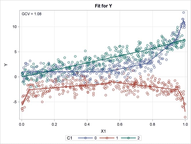
Output 24.2.2 displays the fitted linear splines overlaid with the original data. PROC ADAPTIVEREG captures the three underlying data-generating
processes. For observations with C1 at level 0, the shape of the fitted splines is quite similar to the exponential function. For observations with C1 at level 1, the shape of the fitted spline suggests a symmetric function along X1 with a symmetry point approximately equal to 0.5. The function at each side of the symmetry point is analogous to the logarithmic
transformation. For the rest of the observations with C1 at level 2, PROC ADAPTIVEREG suggests a strict linear model. The fitted model is very close to the true model. PROC ADAPTIVEREG
fits the model in an automatic and adaptive way, except that it needs the CLASS statement to name the classification variable.
You might notice that some basis functions have their parent basis functions not listed in the parameter estimates table (Output 24.2.1). This is because their parent basis functions are dropped during the model selection process. You can view the complete set of basis functions used in the model selection by specifying the DETAILS=BASES option in the PROC ADAPTIVEREG statement, as in the following statements:
proc adaptivereg data=Mixture details=bases;
   class c1;
   model y=c1 x1;
run;
Output 24.2.3: Basis Function Information
| Basis Information | |
|---|---|
| Name | Transformation |
| Basis0 | None |
| Basis1 | Basis0*(C1 = 1 OR C1 = 0) |
| Basis2 | Basis0*NOT(C1 = 1 OR C1 = 0) |
| Basis3 | Basis0*(C1 = 1) |
| Basis4 | Basis0*NOT(C1 = 1) |
| Basis5 | Basis4*MAX(X1 - 0.7665019053,0) |
| Basis6 | Basis4*MAX(0.7665019053 - X1,0) |
| Basis7 | Basis2*MAX(X1 - 0.7665019053,0) |
| Basis8 | Basis2*MAX(0.7665019053 - X1,0) |
| Basis9 | Basis3*MAX(X1 - 0.5530566455,0) |
| Basis10 | Basis3*MAX(0.5530566455 - X1,0) |
| Basis11 | Basis3*MAX(X1 - 0.045800759,0) |
| Basis12 | Basis3*MAX( 0.045800759 - X1,0) |
| Basis13 | Basis3*MAX(X1 - 0.9526330293,0) |
| Basis14 | Basis3*MAX(0.9526330293 - X1,0) |
| Basis15 | Basis1*MAX(X1 - 0.9499325226,0) |
| Basis16 | Basis1*MAX(0.9499325226 - X1,0) |
| Basis17 | Basis1*MAX(X1 - 0.5142821095,0) |
| Basis18 | Basis1*MAX(0.5142821095 - X1,0) |
| Basis19 | Basis1*MAX(X1 - 0.9889635476,0) |
| Basis20 | Basis1*MAX(0.9889635476 - X1,0) |
You can produce a SAS DATA step for scoring new observations by using the information provided in the parameter estimate table and the basis information table, as shown in the following statements:
data New;
   basis1  = (c1=1 OR c1=0);
   basis3  = (c1=1);
   basis5  = NOT(c1=1)*MAX(x1-0.7665019053,0);
   basis7  = NOT(c1=1 OR c1=0)*MAX(x1-0.7665019053,0);
   basis8  = NOT(c1=1 OR c1=0)*MAX(0.7665019053-x1,0);
   basis9  = (c1=1)*MAX(x1-0.5530566455,0);
   basis10 = (c1=1)*MAX(0.5530566455-x1,0);
   basis11 = (c1=1)*MAX(x1-0.045800759,0);
   basis13 = (c1=1)*MAX(x1-0.9526330293,0);
   basis15 = (c1=1 OR c1=0)*MAX(x1-0.9499325226,0);
   basis17 = (c1=1 OR c1=0)*MAX(x1-0.5142821095,0);
   basis19 = (c1=1 OR c1=0)*MAX(x1-0.9889635476,0);
   pred    = 5.3829 - 4.3871*basis1 + 32.7761*basis3 +
             20.2859*basis5 - 11.4183*basis7 - 7.0758*basis8 +
             58.4911*basis9 - 71.6388*basis10 - 69.0764*basis11 -
             119.71*basis13 + 66.5733*basis15 + 6.6681*basis17 -
             185.21*basis19;
run;