The ADAPTIVEREG Procedure (Experimental)

This example shows how you can use PROC ADAPTIVEREG to fit a surface model from a data set that contains many nuisance variables.
Consider a simulated data set that contains a response variable and 10 continuous predictors. Each continuous predictor is
sampled independently from the uniform distribution ![]() . The true model is formed by
. The true model is formed by ![]() and
and ![]() :
:
The values of the response variable are generated by adding errors from the standard normal distribution ![]() to the true model. The generating mechanism is adapted from Gu et al. (1990). There are 400 generated observations in all. The following statements create an artificial data set:
to the true model. The generating mechanism is adapted from Gu et al. (1990). There are 400 generated observations in all. The following statements create an artificial data set:
data artificial;
   drop i;
   array X{10};
   do i=1 to 400;
      do j=1 to 10;
         X{j} = ranuni(1);
      end;
      Y = 40*exp(8*((X1-0.5)**2+(X2-0.5)**2))/
            (exp(8*((X1-0.2)**2+(X2-0.7)**2))+
             exp(8*((X1-0.7)**2+(X2-0.2)**2)))+rannor(1);
     output;
   end;
run;
The standard deviation for the response without noise is 3, whereas the standard deviation for the error term is 1. So the
response variable Y has a signal-to-noise ratio of 3. When eight more variables are introduced, it is harder to search for the true model because
of the extra variability that the nuisance variables create. The objective is to fit a nonparametric surface model that can
well approximate the true model without experiencing much interference from the nuisance variables.
The following statements invoke the ADAPTIVEREG procedure to fit the model:
ods graphics on;

proc adaptivereg data=artificial plots=fit;
   model y=x1-x10;
run;
The PLOTS=FIT option in the PROC ADAPTIVEREG statement requests a fit plot. PROC ADAPTIVEREG might not produce the fit plot because the number of predictors in the final model is unknown. If the final model has no more than two variables, then the fit can be graphically presented.
PROC ADAPTIVEREG selects the two variables that form the true model (X1, X2) and does not include other nuisance variables. The “Fit Statistics” table (Output 24.1.1) lists summary statistics of the fitted surface model. The model has 27 effective degrees of freedom and 14 basis functions
formed by X1 or X2 or both. The fit statistics suggest that this is a reasonable fit.
Output 24.1.1: Fit Statistics
| Fit Statistics | |
|---|---|
| GCV | 1.55656 |
| GCV R-Square | 0.86166 |
| Effective Degrees of Freedom | 27 |
| R-Square | 0.87910 |
| Adjusted R-Square | 0.87503 |
| Mean Square Error | 1.40260 |
| Average Square Error | 1.35351 |
Output 24.1.2 lists both parameter estimates and construction components (parent basis function, new variable, and optimal knot for the new variable) for the basis functions.
Output 24.1.2: Parameter Estimates
| Regression Spline Model after Backward Selection | ||||
|---|---|---|---|---|
| Name | Coefficient | Parent | Variable | Knot |
| Basis0 | 12.3031 | Intercept | ||
| Basis1 | 13.1804 | Basis0 | X1 | 0.05982 |
| Basis3 | -23.4892 | Basis0 | X2 | 0.1387 |
| Basis4 | -171.03 | Basis0 | X2 | 0.1387 |
| Basis5 | -86.1867 | Basis3 | X1 | 0.6333 |
| Basis7 | -436.86 | Basis4 | X1 | 0.5488 |
| Basis8 | 397.18 | Basis4 | X1 | 0.5488 |
| Basis9 | 11.4682 | Basis1 | X2 | 0.6755 |
| Basis10 | -19.1796 | Basis1 | X2 | 0.6755 |
| Basis13 | 126.84 | Basis11 | X1 | 0.6018 |
| Basis14 | 40.8134 | Basis11 | X1 | 0.6018 |
| Basis15 | 22.2884 | Basis0 | X1 | 0.7170 |
| Basis17 | -53.8746 | Basis12 | X1 | 0.2269 |
| Basis19 | 598.89 | Basis4 | X1 | 0.2558 |
Output 24.1.3 shows all the ANOVA functional components that form the final model. The function estimate consists of two basis functions
for each of X1 and X2 and nine bivariate functions of both variables. Because the true model contains the interaction between X1 and X2, PROC ADAPTIVEREG automatically selects many interaction terms.
Output 24.1.3: ANOVA Decomposition
| ANOVA Decomposition | ||||
|---|---|---|---|---|
| Functional Component |
Number of Bases |
DF | Change If Omitted | |
| Lack of Fit | GCV | |||
| X1 | 2 | 4 | 405.18 | 1.1075 |
| X2 | 2 | 4 | 947.87 | 2.6348 |
| X2 X1 | 9 | 18 | 2583.21 | 6.6187 |
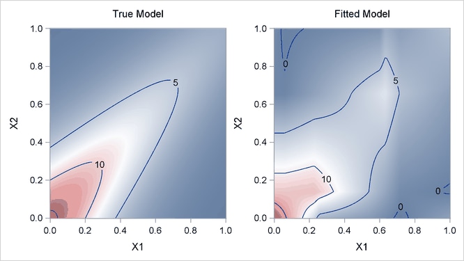
To compute predictions for the contour plot of the fitted model, you can use the SCORE statement. The following statements produce the graph that shows both the true model and the fitted model:
data score;
   do X1=0 to 1 by 0.01;
      do X2=0 to 1 by 0.01;
         Y=40*exp(8*((X1-0.5)**2+(X2-0.5)**2))/
             (exp(8*((X1-0.2)**2+(X2-0.7)**2))+
              exp(8*((X1-0.7)**2+(X2-0.2)**2)));
         output;
      end;
   end;
run;
proc adaptivereg data=artificial;
   model y=x1-x10;
   score data=score out=scoreout;
run;

proc template;
   define statgraph surfaces;
   begingraph / designheight=360px;
      layout lattice/columns=2;
         layout overlay/xaxisopts=(offsetmin=0 offsetmax=0)
                        yaxisopts=(offsetmin=0 offsetmax=0);
            entry "True Model" / location=outside valign=top
                                 textattrs=graphlabeltext;
            contourplotparm z=y y=x2 x=x1;
         endlayout;
         layout overlay/xaxisopts=(offsetmin=0 offsetmax=0)
                        yaxisopts=(offsetmin=0 offsetmax=0);
            entry "Fitted Model" / location=outside valign=top
                                 textattrs=graphlabeltext;
            contourplotparm z=pred y=x2 x=x1;
         endlayout;
      endlayout;
   endgraph;
end;

proc sgrender data=scoreout template=surfaces;
run;
Output 24.1.4 displays surfaces for both the true model and the fitted model. The fitted model approximates the underlying true model well.
For high-dimensional data sets with complex underlying data-generating mechanisms, many different models can almost equally approximate the true mechanisms. Because of the sequential nature of the selection mechanism, any change in intermediate steps due to perturbations from local structures might yield completely different models. Therefore, PROC ADAPTIVEREG might find models that contain noisy variables. For example, if you change the random number seed in generating the data (as in the following statements), PROC ADAPTIVEREG might return different models with more variables. You can use the information from the variable importance table (Output 24.1.5) to aid further analysis.
data artificial;
   drop i;
   array x{10};
   do i=1 to 400;
      do j=1 to 10;
         x{j} = ranuni(12345);
      end;
      y = 40*exp(8*((x1-0.5)**2+(x2-0.5)**2))/
            (exp(8*((x1-0.2)**2+(x2-0.7)**2))+
             exp(8*((x1-0.7)**2+(x2-0.2)**2)))+rannor(1);
      output;
   end;
run;
proc adaptivereg data=artificial;
   model y=x1-x10;
run;
Output 24.1.5 shows that the variables X1 and X2 are two dominating factors for predicting the response, whereas the relative importance of the variable X8 compared to the other two is negligible. You might want to remove the variable if you fit a new model.
Output 24.1.5: Variable Importance
| Variable Importance | ||
|---|---|---|
| Variable | Number of Bases |
Importance |
| x1 | 13 | 100.00 |
| x2 | 12 | 98.58 |
| x8 | 2 | 0.22 |