The KRIGE2D Procedure

Example 49.2 Investigating the Effect of Model Specification on Spatial Prediction
It is generally believed that spatial prediction is robust against model specification, while the standard error computation is not so robust. This example investigates the effect of using these different models on the prediction and associated standard errors.
In the section Theoretical Semivariogram Model Fitting in the VARIOGRAM procedure, a particular theoretical semivariogram is fitted to the coal seam thickness data empirical semivariogram.
The chosen semivariogram is Gaussian with a scale (sill) of ![]() and a range of
and a range of ![]() .
.
Another possible model choice could be the spherical semivariogram. First, use a DATA step to input the thickness data:
title 'Effect of Model Specification on Prediction';

data thick;
   input East North Thick @@;
   label Thick='Coal Seam Thickness';
   datalines;
    0.7  59.6  34.1   2.1  82.7  42.2   4.7  75.1  39.5
    4.8  52.8  34.3   5.9  67.1  37.0   6.0  35.7  35.9
    6.4  33.7  36.4   7.0  46.7  34.6   8.2  40.1  35.4
   13.3   0.6  44.7  13.3  68.2  37.8  13.4  31.3  37.8
   17.8   6.9  43.9  20.1  66.3  37.7  22.7  87.6  42.8
   23.0  93.9  43.6  24.3  73.0  39.3  24.8  15.1  42.3
   24.8  26.3  39.7  26.4  58.0  36.9  26.9  65.0  37.8
   27.7  83.3  41.8  27.9  90.8  43.3  29.1  47.9  36.7
   29.5  89.4  43.0  30.1   6.1  43.6  30.8  12.1  42.8
   32.7  40.2  37.5  34.8   8.1  43.3  35.3  32.0  38.8
   37.0  70.3  39.2  38.2  77.9  40.7  38.9  23.3  40.5
   39.4  82.5  41.4  43.0   4.7  43.3  43.7   7.6  43.1
   46.4  84.1  41.5  46.7  10.6  42.6  49.9  22.1  40.7
   51.0  88.8  42.0  52.8  68.9  39.3  52.9  32.7  39.2
   55.5  92.9  42.2  56.0   1.6  42.7  60.6  75.2  40.1
   62.1  26.6  40.1  63.0  12.7  41.8  69.0  75.6  40.1
   70.5  83.7  40.9  70.9  11.0  41.7  71.5  29.5  39.8
   78.1  45.5  38.7  78.2   9.1  41.7  78.4  20.0  40.8
   80.5  55.9  38.7  81.1  51.0  38.6  83.8   7.9  41.6
   84.5  11.0  41.5  85.2  67.3  39.4  85.5  73.0  39.8
   86.7  70.4  39.6  87.2  55.7  38.8  88.1   0.0  41.6
   88.4  12.1  41.3  88.4  99.6  41.2  88.8  82.9  40.5
   88.9   6.2  41.5  90.6   7.0  41.5  90.7  49.6  38.9
   91.5  55.4  39.0  92.9  46.8  39.1  93.4  70.9  39.7
   55.8  50.5  38.1  96.2  84.3  40.3  98.2  58.2  39.5
   ;
Fitting of the Gaussian model is performed in the section Theoretical Semivariogram Model Fitting in the VARIOGRAM procedure, and the fitting parameters are saved in the SemivStoreGau item store with the following statements:
ods graphics on;
proc variogram data=thick noprint;
   store out=SemivStoreGau / label='Thickness Gaussian Model';
   compute lagd=7 maxlag=10;
   coord xc=East yc=North;
   model form=gau;
   var Thick;
run;
For prediction with the saved Gaussian model, you use the following statements to run the KRIGE2D procedure with input from
the SemivStoreGau item store. You invoke the item store with the RESTORE statement. The STORESELECT option in the MODEL statement that specifies that you want to use the selected model in the item store as input for your prediction.
proc krige2d data=thick outest=pred1 noprint;
   restore in=SemivStoreGau;
   coordinates xc=East yc=North;
   predict var=Thick r=60;
   model storeselect;
   grid x=0 to 100 by 10 y=0 to 100 by 10;
run;
Then, you run the KRIGE2D procedure by using a spherical model. Start by using the VARIOGRAM procedure to fit a spherical
model to the thick data set empirical semivariogram. You specify the STORE statement again in PROC VARIOGRAM to save the spherical model estimated
parameters in an item store with the name SemivStoreSph. You use the following statements:
proc variogram data=thick plots(only)=fit;
   store out=SemivStoreSph / label='Thickness Sph Model';
   compute lagd=7 maxlag=10;
   coord xc=East yc=North;
   model form=sph;
   var Thick;
run;
The VARIOGRAM procedure fits the spherical model successfully, and the estimated parameters for this fit are shown in Output 49.2.1.
Output 49.2.1: Spherical Model Fitting Parameter Estimates
| Effect of Model Specification on Prediction |
| Parameter Estimates | |||||
|---|---|---|---|---|---|
| Parameter | Estimate | Approx Std Error |
DF | t Value | Approx Pr > |t| |
| Nugget | 0 | 0 | 8 | . | . |
| Scale | 7.1914 | 0.2827 | 8 | 25.44 | <.0001 |
| Range | 63.2351 | 4.1050 | 8 | 15.40 | <.0001 |
The fit summary is displayed in Output 49.2.2. When compared to the corresponding result in the section Theoretical Semivariogram Model Fitting in the VARIOGRAM procedure, the goodness-of-fit criteria indicate a worse statistical fit for the spherical model compared to the Gaussian.
Output 49.2.2: Spherical Model Fit Summary
| Fit Summary | ||
|---|---|---|
| Model | Weighted SSE |
AIC |
| Sph | 52.26791 | 23.14336 |
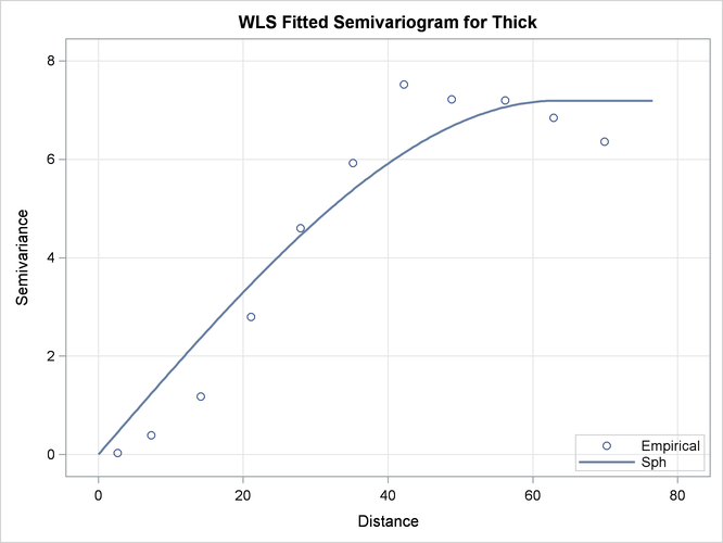
Output 49.2.3 suggests an acceptable fit of the spherical model to the thick data set. Obviously, the fit of the spherical model in the sensitive area near the semivariogram origin is less faithful
to the empirical semivariance than the Gaussian model. The following analysis explores the consequence in the kriging prediction
of this discrepancy.
Output 49.2.3: Fitted Spherical and Empirical Thick Semivariogram
For the next step, you run the KRIGE2D procedure by using the spherical model parameters stored in the SemivStoreSph item store. You use the following statements:
proc krige2d data=thick outest=pred2 noprint;
   restore in=SemivStoreSph;
   coordinates xc=East yc=North;
   predict var=Thick r=60;
   model storeselect;
   grid x=0 to 100 by 10 y=0 to 100 by 10;
run;
Eventually, you compare the prediction results and errors of the two models. You use a DATA step to compute the relative difference
of the predicted values and the prediction error for each one of the Gaussian and the spherical models. You store the prediction
relative difference in the prdRelDiff variable and the prediction relative error in the stdRelDiff variable. You save the output in the compare data set with the following statements:
data compare;
   merge pred1(rename=(estimate=g_prd stderr=g_std))
         pred2(rename=(estimate=s_prd stderr=s_std));
   prdRelDif = ((g_prd-s_prd) / s_prd) * 100;
   stdRelDif = ((g_std-s_std) / s_std) * 100;
run;
The MEANS procedure uses the compare data set to produce statistics about the prediction relative difference and error for each one of the prdRelDiff and stdRelDiff variables with the following statements:
proc means data=compare;
   var prdRelDif stdRelDif;
run;

ods graphics off;
Output 49.2.4 shows that on average the predicted values are very close for the two semivariogram models. The mean relative difference in the prediction values is close to zero with a low standard deviation, whereas the relative difference values fluctuate with an absolute maximum of about 5%.
However, note that the mean relative standard error is about -96%. According to the definition of the stdRelDiff variable, the high negative value indicates that the prediction error difference between the two models is very close to
the spherical model prediction error. Hence, the prediction standard error of the spherical model is substantially larger
than that of the Gaussian model. In fact, the prediction relative error never gets smaller than about 66% for the two models,
where the negative sign in the Minimum and Maximum columns in Output 49.2.4 means that the prediction error is always greater for the spherical model.
Output 49.2.4: Comparison of Gaussian and Spherical Models
| Effect of Model Specification on Prediction |
| Variable | N | Mean | Std Dev | Minimum | Maximum | ||||||||||||
|---|---|---|---|---|---|---|---|---|---|---|---|---|---|---|---|---|---|
|
|
|
|
|
|