The KRIGE2D Procedure

Example 49.1 Spatial Prediction of Pollutant Concentration
The example in the section Aspects of Semivariogram Model Fitting in the VARIOGRAM procedure investigates fitting of a theoretical model to describe spatial correlation in a study of 138
simulated arsenic logarithm concentration (logAs) observations. These observations form the logAsData data set, which is treated as actual data for illustration in the examples.
In this example, you use the logAsData data set and the semivariogram analysis results to predict the logAs variable values across space in a specified square region of size 500 km ![]() 500 km. Your goal is to answer scientific questions in your analysis by means of your prediction results. This application
highlights the impact of the correlation model choice on predictions. The example in section Investigating the Effect of Model Specification on Spatial Prediction examines additional aspects of this impact.
500 km. Your goal is to answer scientific questions in your analysis by means of your prediction results. This application
highlights the impact of the correlation model choice on predictions. The example in section Investigating the Effect of Model Specification on Spatial Prediction examines additional aspects of this impact.
The World Health Organization (WHO) standard for maximum arsenic concentration in drinking water is 10 ![]() g/lt. Assume that you want to answer the following question: In what percentage of the study area does the Arsenic concentration
exceed the WHO regulatory standard?
g/lt. Assume that you want to answer the following question: In what percentage of the study area does the Arsenic concentration
exceed the WHO regulatory standard?
First, you read the logAsData data set with the following DATA step:
title 'Spatial Prediction of Log-Arsenic Concentration';

data logAsData;
   input East North logAs @@;
   label logAs='log(As) Concentration';
   datalines;
   193.0 296.6 -0.68153   232.6 479.1  0.96279   268.7 312.5 -1.02908
    43.6   4.9  0.65010   152.6  54.9  1.87076   449.1 395.8  0.95932
   310.9 493.6 -1.66208   287.8 164.9 -0.01779   330.0   8.0  2.06837
   225.7 241.7  0.15899   452.3  83.4 -1.21217   156.5 462.5 -0.89031
    11.5  84.4 -0.24496   144.4 335.7  0.11950   149.0 431.8 -0.57251
   234.3 123.2 -1.33642    37.8 197.8 -0.27624   183.1 173.9 -2.14558
   149.3 426.7 -1.06506   434.4  67.5 -1.04657   439.6 237.0 -0.09074
    36.4 175.2 -1.21211   370.6 244.0  3.28091   452.0  96.5 -0.77081
   247.0  86.8  0.04720   413.6 373.2  1.78235   253.5 291.7  0.56132
   129.7 111.9  1.34000   352.7  42.1  0.23621   279.3  82.7  2.12350
   382.6 290.7  0.86756   188.2 222.8 -1.23308   382.8 154.5 -0.94094
   304.4 309.2 -1.95158   337.5 387.2 -1.31294   490.7 189.8  0.40206
   159.0 100.1 -0.22272   245.5 329.2 -0.26082   372.1 379.5 -1.89078
   417.8  84.1 -1.25176   173.9 407.6 -0.24240   121.5 107.7  1.54509
   453.5 313.6  0.65895   143.5 346.7 -0.87196   157.4 125.5 -1.96165
   371.8 353.2 -0.59464   358.9 338.2 -1.07133     8.6 437.8  1.44203
   395.9 394.2 -0.24144   149.5  58.9  1.17459   453.5 420.6 -0.63951
   182.3  85.0  1.00005    21.0 290.1  0.31016    11.1 352.2 -0.88418
   131.2 238.4 -0.57184   104.9   6.3  1.12054   247.3 256.0  0.14019
   428.4 383.7  0.92448   327.8 481.1 -2.72543   199.2  92.8 -0.05717
   453.9 230.1  0.16571   205.0 250.6  0.07581   459.5 271.6  0.93700
   229.5 262.8  1.83590   370.4 228.6  2.96611   330.2 281.9  1.79723
   354.8 388.3 -3.18262   406.2 222.7  2.41594   254.4 393.1  2.03221
    96.7  85.2 -0.47156   407.2 256.8  0.66747   498.5 273.8  1.03041
   417.2 471.4 -1.42766   368.8 424.3 -0.70506   303.0  59.1  1.43070
   403.1 264.1  1.64554    21.2 360.8  0.67094   148.2  78.1  2.15323
   305.5 310.7 -1.47985   228.5 180.3 -0.68386   161.1 143.3  1.07901
    70.5 155.1  0.54652   363.1 282.6 -0.43051    86.0 472.5 -1.18855
   175.9 105.3 -2.08112    96.8 426.3  1.56592   475.1 453.1 -1.53776
   125.7 485.4  1.40054   277.9 201.6 -0.54565   406.2 125.0 -1.38657
    60.0 275.5 -0.59966   431.3 494.6 -0.36860   399.9 399.0 -0.77265
    28.8 311.1  0.91693   166.1 348.2 -0.49056   266.6  83.5  0.67277
    54.7 356.3  0.49596   433.5 460.3 -1.61309   201.7 167.6 -1.40678
   158.1 203.6 -1.32499    67.6 230.4  1.14672    81.9 250.0  0.63378
   372.0  50.7  0.72445    26.4 264.6  1.00862   300.1  91.7 -0.74089
   303.0 447.4  1.74589   108.4 386.2  1.12847    55.6 191.7  0.95175
    36.3 273.2  1.78880    94.5 298.3 -2.43320   366.1 187.3 -0.80526
   130.7 389.2 -0.31513    37.2 324.2  0.24489   295.5 211.8  0.41899
    58.6 206.2  0.18495   346.3 142.8 -0.92038   484.2 215.9  0.08012
   451.4 415.7  0.02773    58.9  86.5  0.17652   212.6 363.9  0.17215
   378.7 407.6  0.51516   265.9 305.0 -0.30718   123.2 314.8 -0.90591
    26.9 471.7  1.70285    16.5   7.1  0.51736   255.1 472.6  2.02381
   111.5 148.4 -0.09658   440.4 375.0  1.23285   406.4  19.5  1.01181
   321.2  65.8 -0.02095   466.4 357.1 -0.49272     2.0 484.6  0.50994
   200.9 205.1  0.43543    30.3 337.0  1.60882   297.0  12.7  1.79824
   158.2 450.7  0.05295   122.8 105.3  1.53936   417.8 329.7 -2.08124
   ;
For prediction of the logAs values in the specified area, assume a rectangular grid of nodes with an equal spacing of 5 km between neighboring nodes
in the north and east directions. This produces a total of ![]() prediction locations.
prediction locations.
In the section Aspects of Semivariogram Model Fitting in the VARIOGRAM procedure, you saved the selected fitted model that resulted from the correlation analysis into the SemivAsStore item store as shown in the following statements:
ods graphics on;
proc variogram data=logAsData plots=none;
   store out=SemivAsStore / label='LogAs Concentration Models';
   compute lagd=5 maxlag=40;
   coord xc=East yc=North;
   model form=auto(mlist=(exp,gau,mat) nest=1 to 2);
   var logAs;
run;
In the KRIGE2D procedure you specify the name of the item store you want to use for prediction input in the IN= option of the RESTORE statement. You request use of the selected model for prediction by specifying the STORESELECT option in the MODEL statement.
The INFO option of the RESTORE statement produces a table with information about the selected fitted model in the item store. To review all models in the input item store, specify the two INFO option suboptions. In particular, specify the DET suboption to request details about all additional fitted models that are included in the item store and the ONLY suboption to suppress prediction and produce only the tables about the item store, as shown in the following statements:
proc krige2d data=logAsData outest=pred plots=none;
   restore in=SemivAsStore / info(det only);
   coordinates xc=East yc=North;
   predict var=logAs;
   model storeselect;
   grid x=0 to 500 by 5 y=0 to 500 by 5;
run;
PROC KRIGE2D produces a table with general information about the input item store identity, as shown in Output 49.1.1.
Output 49.1.1: PROC KRIGE2D and Input Item Store General Information
| Spatial Prediction of Log-Arsenic Concentration |
| Correlation Model Item Store Information | |
|---|---|
| Input Item Store | WORK.SEMIVASSTORE |
| Item Store Label | LogAs Concentration Models |
| Data Set Created From | WORK.LOGASDATA |
| By-group Information | No By-groups Present |
| Created By | PROC VARIOGRAM |
| Date Created | 07JUN12:11:31:33 |
The second table in Output 49.1.2 itemizes the variables in the item store and displays the sample mean and standard deviation of their data set of origin.
Hence, the values shown in Output 49.1.2 refer to the observations in the logAsData data set.
Output 49.1.2: Variables in the Input Item Store
| Item Store Variables | ||
|---|---|---|
| Variable | Mean | Std Deviation |
| logAs | 0.084309 | 1.527707 |
The table in Output 49.1.3 presents all the correlation models fitted to the arsenic logarithm logAs empirical semivariance that are saved in the SemivAsStore item store.
Output 49.1.3: Angle and Models Information in the Input Item Store
| Item Store Models For logAs |
|
|---|---|
| Class | Model |
| 1 | Gau-Gau |
| Gau-Mat | |
| 2 | Exp-Gau |
| 3 | Exp-Mat |
| 4 | Mat |
| 5 | Gau |
| 6 | Exp |
| Exp-Exp | |
| Mat-Exp | |
| Gau-Exp | |
According to Output 49.1.3, the Gaussian-Gaussian model is the selected model for the empirical semivariance fit based on the specific weighted least
squares fit and ranking criteria. In the section Aspects of Semivariogram Model Fitting in the VARIOGRAM procedure, it is noted that all fitted models in the first five equivalence classes produce very similar
semivariograms, and this is likely to lead to similar results in prediction analysis. For comparison purposes, you choose
to examine the selected model, in addition to the exponential model in the SemivAsStore item store. As shown in Output 49.1.3, the exponential model is one of the least well-fit models based on the criteria used for the specific fit. You are interested
in comparing the predictions from each one of these two models, and you examine their impact on your analysis.
The default item store model selection is the model on top of the list in Output 49.1.3. Hence, you specify the STORESELECT option in the MODEL statement without any suboptions, and it invokes the Gaussian-Gaussian model from the SemivAsStore item store. You assign the label SELMODEL to the corresponding MODEL statement.
You also specify a second MODEL statement with the label EXPMODEL to request prediction based on the exponential correlation form. In this case you specify the STORESELECT(MODEL=) option in the MODEL statement to request the desired form.
You omit the INFO option from the RESTORE statement. You specify the PRED and the SEMIVAR options in the PLOTS option of the PROC KRIGE2D statement to produce plots of the predicted values and the semivariance model, respectively, for each MODEL statement. You request that the prediction output be saved in the Pred output data set.
You satisfy the preceding requests by specifying the following statements:
proc krige2d data=logAsData outest=Pred plots(only)=(pred semivar);
   restore in=SemivAsStore;
   coordinates xc=East yc=North;
   predict var=logAs;
   SelModel: model storeselect;
   ExpModel: model storeselect(model=exp);
   grid x=0 to 500 by 5 y=0 to 500 by 5;
run;
When you run these statements, in addition to the input item store information table, PROC KRIGE2D also produces the number of observations table and general kriging process information, as shown in Output 49.1.4.
Output 49.1.4: Number of Observations and Kriging Information Tables
| Spatial Prediction of Log-Arsenic Concentration |
| Number of Observations Read | 138 |
|---|---|
| Number of Observations Used | 138 |
| Kriging Information | |
|---|---|
| Prediction Grid Points | 10201 |
| Type of Analysis | Global |
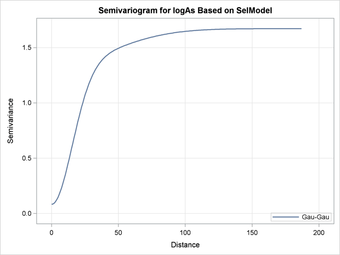
PROC KRIGE2D first uses the Gaussian-Gaussian model. The table in Output 49.1.5 shows the saved parameter values of the fitted Gaussian-Gaussian model in the SemivAsStore item store. PROC KRIGE2D uses these parameters for the prediction based on the selected model.
Output 49.1.5: Information about the Gaussian-Gaussian Model
| Spatial Prediction of Log-Arsenic Concentration |
| Covariance Model Information for SelModel | |
|---|---|
| Nested Structure 1 Type | Gaussian |
| Nested Structure 1 Sill | 0.3276646 |
| Nested Structure 1 Range | 62.312728 |
| Nested Structure 1 Effective Range | 107.92881 |
| Nested Structure 2 Type | Gaussian |
| Nested Structure 2 Sill | 1.261545 |
| Nested Structure 2 Range | 21.459563 |
| Nested Structure 2 Effective Range | 37.169053 |
| Nugget Effect | 0.0830758 |
The semivariogram of the Gaussian-Gaussian model with the parameters shown in Output 49.1.5 is depicted in Output 49.1.6.
Output 49.1.6: Gaussian-Gaussian Semivariogram Model Used in Kriging Predictions
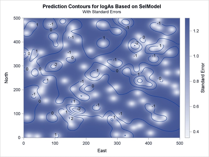
Output 49.1.7 is a map of the kriging prediction of the arsenic concentration values logAs in the specified domain. The prediction error surface shows a naturally increasing error as you move farther away from the
observation locations. Interestingly, kriging predicts a small area of increased arsenic concentration values located in the
central-eastern part of the domain. The WHO threshold of 10 ![]() g/lt for the maximum allowed arsenic concentration in water translates into about 2.3 in the log scale, and the particular
area exhibits values in excess of 3. Due to the suggested violation of the WHO standard, this particular area is very likely
to be the focus of further environmental risk analysis.
g/lt for the maximum allowed arsenic concentration in water translates into about 2.3 in the log scale, and the particular
area exhibits values in excess of 3. Due to the suggested violation of the WHO standard, this particular area is very likely
to be the focus of further environmental risk analysis.
Output 49.1.7: Predicted Arsenic Logarithm Values with Gaussian-Gaussian Covariance
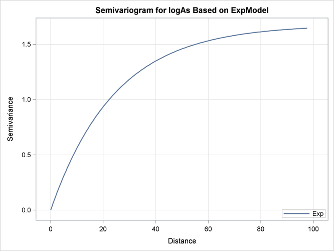
Next, PROC KRIGE2D performs prediction with the exponential model. The model parameters are also read from the SemivAsStore item store and are shown in Output 49.1.8.
Output 49.1.8: Information about the Exponential Model
| Spatial Prediction of Log-Arsenic Concentration |
| Covariance Model Information for ExpModel |
|
|---|---|
| Type | Exponential |
| Sill | 1.6779788 |
| Range | 24.537294 |
| Effective Range | 73.611882 |
| Nugget Effect | 0 |
Output 49.1.9 illustrates the semivariogram of the nested exponential model where its parameter values are those shown in Output 49.1.8.
Output 49.1.9: Exponential Semivariogram Model Used in Kriging Predictions
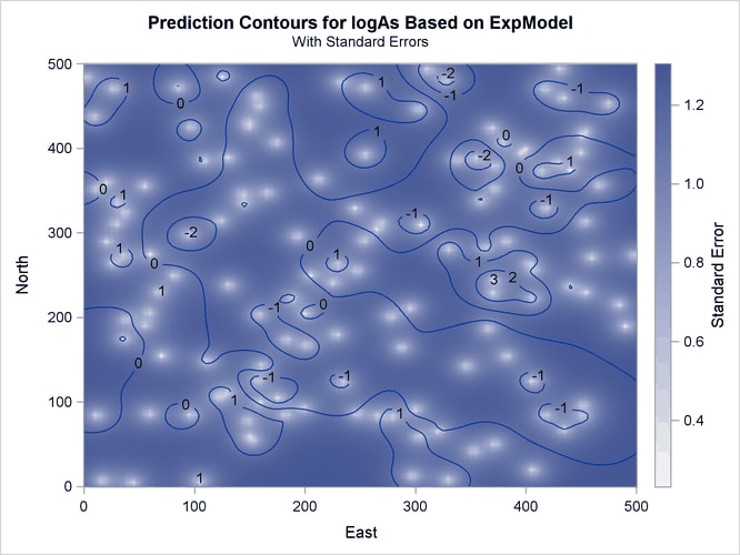
The prediction plot for the exponential model is shown in Output 49.1.10. Prediction values and spatial patterns are similar overall to those of the Gaussian-Gaussian case. Clearly, although both models predict the same basic characteristics for the arsenic logarithm concentration distribution, the exponential model suggests a more limited spatial variability in closely neighboring locations. The lack of a nugget effect in the exponential model justifies this behavior. Also, the exponential model predictions seem less inclined to deviate farther away from the near-zero mean than the Gaussian-Gaussian model predictions.The prediction error reaches about the same upper values for both models, though its low values are slightly smaller in the exponential model.
Output 49.1.10: Predicted Arsenic Logarithm Values with Exponential Covariance
In the following two-step computation, you proceed to compute the percentage of the study area where the arsenic concentration
exceeds the WHO regulatory standard according to your predictions. First, a DATA step marks the arsenic predicted values in
excess of the WHO concentration threshold of 10 ![]() g/lt and saves the outcome into an indicator variable
g/lt and saves the outcome into an indicator variable OverLimit. The DATA step input is the prediction Pred output data set, where the logarithm arsenic prediction is stored in the estimate variable. The DATA step also transforms the arsenic logarithm values back into arsenic concentration values to compare them
to the threshold value. You use the following statements:
data AsOverLimit;
   set Pred;
   OverLimit = (exp(estimate) > 10) * 100;
run;
The second step uses the MEANS procedure to express the selected nodes population, where the WHO arsenic concentration limit
violation occurs, as a percentage of the entire domain area. You study the results of each correlation model separately by
specifying the BY statement in the PROC MEANS. The BY variable is the Label variable in the AsOverLimit and Pred data sets. You need to sort the AsOverLimit data prior to using PROC MEANS. You run the following statements:
proc sort data=AsOverLimit;
   by Label;
run;
proc means data=AsOverLimit mean;
   var OverLimit;
   by label;
   label Overlimit="Percent above WHO threshold";
run;

ods graphics off;
The Gaussian-Gaussian model prediction produces the result in Output 49.1.11. The analysis suggests a minimal occurrence of excessive arsenic concentration in drinking water in about 0.43% of the study region.
Output 49.1.11: Violation of Arsenic Concentration Threshold Using Gaussian-Gaussian Model
| Spatial Prediction of Log-Arsenic Concentration |
| Analysis Variable : OverLimit Percent above WHO threshold |
|---|
| Mean |
| 0.4313303 |
The exponential model predicts that the WHO arsenic concentration threshold is exceeded in about 0.27% of the domain, as shown in Output 49.1.12. Although this is still a minimal occurrence of the threshold violation across the region, the exponential model estimates the impact to be at about two thirds of the Gaussian-Gaussian model percentage.
Output 49.1.12: Violation of Arsenic Concentration Threshold Using Exponential Model
| Spatial Prediction of Log-Arsenic Concentration |
| Analysis Variable : OverLimit Percent above WHO threshold |
|---|
| Mean |
| 0.2744829 |
The results in Output 49.1.11 and Output 49.1.12 suggest that it might not be possible to provide a unique answer about the area percentage that is affected by increased arsenic concentration. You chose to examine two different correlation models whose performance is relatively similar, and they provide impact estimates that differ by about 37%.
You might conclude that the answer to the initial question about the percentage value lies in the neighborhood of the results given by the two correlation models. Further analysis with more models is necessary to validate this assumption. It is important to note that apart from the continuity model choice, additional factors contribute to this investigation. Such factors could be the use of local instead of global kriging, or even going back to the empirical semivariogram computation stage and repeating the analysis for different possible spatial continuity empirical estimates. A sensible approach to tackle this analysis would be to investigate the range of the impact suggested by all candidate correlation models and to proceed by defining the best and worst case scenarios for the size of the affected area.
Eventually, when it comes to using your findings, it is important to account for the subjective nature of stochastic analysis and multiple possible answers to your questions. In that sense, some scientific questions might be more sensible than others to interpret your results correctly. For instance, you might want to investigate only whether the adversely affected domain percentage is below 1%, rather than attempting to provide a specific value for it. Then, you might consider the preceding findings sufficient, despite any fluctuations in the estimated percentage. In a different scenario, the areas with high pollutant concentration could be populated. Hence, any local health standard violation is probably unacceptable, and it can be crucial that you provide solid and more detailed assessment in that case.
The section Risk Analysis with Simulation in the SIM2D procedure investigates a different aspect of this study and offers additional perspective about spatial analysis.