The GAM Procedure
- Overview
- Getting Started
-
Syntax

-
DetailsMissing ValuesNonparametric RegressionAdditive Models and Generalized Additive ModelsForms of Additive ModelsEstimates from PROC GAMBackfitting and Local Scoring AlgorithmsSmoothersSelection of Smoothing ParametersConfidence Intervals for SmoothersDistribution Family and Canonical LinkDispersion ParameterComputational ResourcesODS Table NamesODS Graphics
-
Examples
- References
Getting Started: GAM Procedure
The following example illustrates the use of the GAM procedure to explore in a nonparametric way how two factors affect a response. The data come from a study of the factors affecting patterns of insulin-dependent diabetes mellitus in children (Sochett et al., 1987). The objective is to investigate the dependence of the level of serum C-peptide on various other factors in order to understand the patterns of residual insulin secretion. The response measurement is the logarithm of C-peptide concentration (pmol/ml) at diagnosis, and the predictor measurements are age and base deficit (a measure of acidity).
title 'Patterns of Diabetes';
data diabetes;
   input Age BaseDeficit CPeptide @@;
   logCP = log(CPeptide);
   datalines;
5.2    -8.1  4.8   8.8  -16.1  4.1  10.5   -0.9  5.2
10.6   -7.8  5.5  10.4  -29.0  5.0   1.8  -19.2  3.4
12.7  -18.9  3.4  15.6  -10.6  4.9   5.8   -2.8  5.6
1.9   -25.0  3.7   2.2   -3.1  3.9   4.8   -7.8  4.5
7.9   -13.9  4.8   5.2   -4.5  4.9   0.9  -11.6  3.0
11.8   -2.1  4.6   7.9   -2.0  4.8  11.5   -9.0  5.5
10.6  -11.2  4.5   8.5   -0.2  5.3  11.1   -6.1  4.7
12.8   -1.0  6.6  11.3   -3.6  5.1   1.0   -8.2  3.9
14.5   -0.5  5.7  11.9   -2.0  5.1   8.1   -1.6  5.2
13.8  -11.9  3.7  15.5   -0.7  4.9   9.8   -1.2  4.8
11.0  -14.3  4.4  12.4   -0.8  5.2  11.1  -16.8  5.1
5.1    -5.1  4.6   4.8   -9.5  3.9   4.2  -17.0  5.1
6.9    -3.3  5.1  13.2   -0.7  6.0   9.9   -3.3  4.9
12.5  -13.6  4.1  13.2   -1.9  4.6   8.9  -10.0  4.9
10.8  -13.5  5.1
;
The following statements perform the desired analysis. The PROC GAM statement invokes the procedure and specifies the diabetes data set as input. The MODEL statement specifies logCP as the response variable and names Age and BaseDeficit as independent variables with univariate smoothing splines and the default of four degrees of freedom.
ods graphics on;
proc gam data=diabetes;
   model logCP = spline(Age) spline(BaseDeficit);
run;
The results are shown in Figure 39.1 and Figure 39.2.
Figure 39.1: Summary Statistics
| Patterns of Diabetes |
| Summary of Input Data Set | |
|---|---|
| Number of Observations | 43 |
| Number of Missing Observations | 0 |
| Distribution | Gaussian |
| Link Function | Identity |
| Iteration Summary and Fit Statistics | |
|---|---|
| Final Number of Backfitting Iterations | 5 |
| Final Backfitting Criterion | 5.542745E-10 |
| The Deviance of the Final Estimate | 0.4180791724 |
Figure 39.1 shows two tables. The first table summarizes the input data set and the distributional family used for the model; the second table summarizes the convergence criterion for backfitting.
Figure 39.2: Analysis of Model
| Regression Model Analysis Parameter Estimates |
||||
|---|---|---|---|---|
| Parameter | Parameter Estimate |
Standard Error |
t Value | Pr > |t| |
| Intercept | 1.48141 | 0.05120 | 28.93 | <.0001 |
| Linear(Age) | 0.01437 | 0.00437 | 3.28 | 0.0024 |
| Linear(BaseDeficit) | 0.00807 | 0.00247 | 3.27 | 0.0025 |
| Smoothing Model Analysis Fit Summary for Smoothing Components |
||||
|---|---|---|---|---|
| Component | Smoothing Parameter |
DF | GCV | Num Unique Obs |
| Spline(Age) | 0.995582 | 3.000000 | 0.011675 | 37 |
| Spline(BaseDeficit) | 0.995299 | 3.000000 | 0.012437 | 39 |
| Smoothing Model Analysis Analysis of Deviance |
||||
|---|---|---|---|---|
| Source | DF | Sum of Squares | Chi-Square | Pr > ChiSq |
| Spline(Age) | 3.00000 | 0.150761 | 12.2605 | 0.0065 |
| Spline(BaseDeficit) | 3.00000 | 0.081273 | 6.6095 | 0.0854 |
Figure 39.2 displays summary statistics for the model. It consists of three tables. The first is the “Parameter Estimates” table for the parametric part of the model. It indicates that the linear trends for both Age and BaseDeficit are highly significant. The second table is the summary of smoothing components of the nonparametric part of the model. This
table presents the smoothing parameter and degrees of freedom (DF) for each component. By default, each smoothing component
has approximately 4 DF. For univariate spline components, one DF is taken up by the (parametric) linear part of the model,
so the remaining approximate DF is 3. Finally, the third table is the “Analysis of Deviance” table for the nonparametric component of the model.
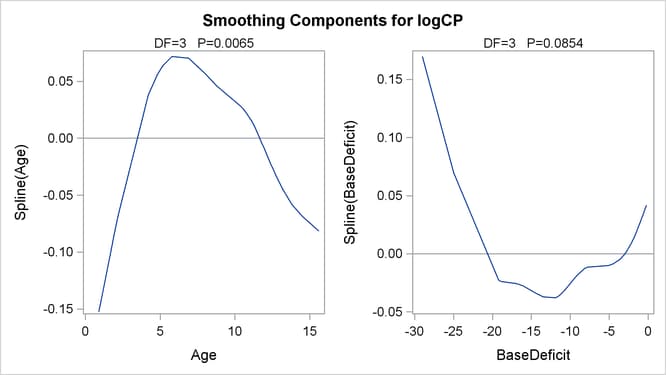
With ODS Graphics enabled, PROC GAM produces by default a panel of plots of partial prediction curves of smoothing components.
In these plots, the partial prediction for a predictor such as Age is its nonparametric contribution to the model, ![]() . For general information about ODS Graphics, see Chapter 21: Statistical Graphics Using ODS. For specific information about the graphics available in the GAM procedure, see the section ODS Graphics.
. For general information about ODS Graphics, see Chapter 21: Statistical Graphics Using ODS. For specific information about the graphics available in the GAM procedure, see the section ODS Graphics.
Plots for both predictors (Figure 39.3) show a strong quadratic pattern, with a possible indication of higher-order behavior. Further investigation is required to determine whether these patterns are real or not.
Figure 39.3: Partial Predictions for Each Predictor