The GAM Procedure
- Overview
- Getting Started
-
Syntax

-
DetailsMissing ValuesNonparametric RegressionAdditive Models and Generalized Additive ModelsForms of Additive ModelsEstimates from PROC GAMBackfitting and Local Scoring AlgorithmsSmoothersSelection of Smoothing ParametersConfidence Intervals for SmoothersDistribution Family and Canonical LinkDispersion ParameterComputational ResourcesODS Table NamesODS Graphics
-
Examples
- References
Backfitting and Local Scoring Algorithms
Much of the development and notation in this section follows Hastie and Tibshirani (1986).
Additive Models
Consider the estimation of the smoothing terms ![]() in the additive model
in the additive model
|
|
where ![]() for every j. Since the algorithm for additive models is the basis for fitting generalized additive models, the algorithm for additive
models is discussed first.
for every j. Since the algorithm for additive models is the basis for fitting generalized additive models, the algorithm for additive
models is discussed first.
Many ways are available to approach the formulation and estimation of additive models. The backfitting algorithm is a general algorithm that can fit an additive model with any regression-type fitting mechanisms.
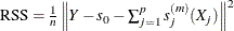
Define the kth set of partial residuals as
|
|
then ![]() . This observation provides a way to estimate each smoothing function
. This observation provides a way to estimate each smoothing function ![]() given estimates
given estimates ![]() for all the others. The resulting iterative procedure is known as the backfitting algorithm (Friedman and Stuetzle, 1981). The following formulation is taken from Hastie and Tibshirani (1986).
for all the others. The resulting iterative procedure is known as the backfitting algorithm (Friedman and Stuetzle, 1981). The following formulation is taken from Hastie and Tibshirani (1986).
The Backfitting Algorithm
The unweighted form of the backfitting algorithm is as follows:
-
Initialization:

-
Iterate:
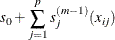
 ;for j = 1 to p do:
  ;
;  ;
;
-
Until:
 fails to decrease, or satisfies the convergence criterion.
In the preceding notation, ![]() denotes the estimate of
denotes the estimate of ![]() at the mth iteration. It can be shown that with many smoothers (including linear regression, univariate and bivariate splines, and
combinations of these), RSS never increases at any step. This implies that the algorithm always converges (Hastie and Tibshirani,
1986). Note, however, that for distributions other than Gaussian, numerical instabilities with weights can cause convergence problems.
Even when the algorithm converges, the individual functions need not be unique, since dependence among the covariates can
lead to more than one representation for the same fitted surface.
at the mth iteration. It can be shown that with many smoothers (including linear regression, univariate and bivariate splines, and
combinations of these), RSS never increases at any step. This implies that the algorithm always converges (Hastie and Tibshirani,
1986). Note, however, that for distributions other than Gaussian, numerical instabilities with weights can cause convergence problems.
Even when the algorithm converges, the individual functions need not be unique, since dependence among the covariates can
lead to more than one representation for the same fitted surface.
A weighted backfitting algorithm has the same form as for the unweighted case, except that the smoothers are weighted. In PROC GAM, weights are used with non-Gaussian data in the local scoring procedure described later in this section.
The GAM procedure uses the following condition as the convergence criterion for the backfitting algorithm:
![\[ \frac{\sum _{i=1}^ n\sum _{j=1}^{p} \left(s^{(m-1)}_ j(\mb {X}_{ij}) - s^{(m)}_ j(\mb {X}_{ij})\right)^2}{1 + \sum _{i=1}^ n\sum _{j=1}^{p} \left(s^{(m-1)}_ j(\mb {X}_{ij})\right)^2}\le \epsilon \]](images/statug_gam0059.png) |
where ![]() by default; you can change this with the EPSILON= option in the MODEL statement.
by default; you can change this with the EPSILON= option in the MODEL statement.
Generalized Additive Models
The algorithm described so far fits only additive models. The algorithm for generalized additive models is a little more
complicated. Generalized additive models extend generalized linear models in the same manner that additive models extend linear
regression models—that is, by replacing the form ![]() with the additive form
with the additive form ![]() . See Generalized Linear Models Theory in Chapter 40: The GENMOD Procedure, for more information.
. See Generalized Linear Models Theory in Chapter 40: The GENMOD Procedure, for more information.
PROC GAM fits generalized additive models by using a modified form of adjusted dependent variable regression, as described for generalized linear models in McCullagh and Nelder (1989), with the additive predictor taking the role of the linear predictor. Hastie and Tibshirani (1986) call this the local scoring algorithm. Important components of this algorithm depend on the link function for each distribution, as shown in the following table.
|
Distribution |
Link |
Adjusted Dependent ( |
Weights ( |
|---|---|---|---|
|
Normal |
|
y |
1 |
|
Binomial |
|
|
|
|
Gamma |
|
|
|
|
Poisson |
|
|
|
|
Inverse Gaussian |
|
|
|
Once the distribution and hence these quantities are defined, the local scoring algorithm proceeds as follows.
The General Local Scoring Algorithm
-
Initialization:

-
Iterate:
 ; Form the predictor
  , mean
  , weights
  , and adjusted dependent variable
  based on their corresponding values from the previous iteration:


![$\displaystyle \left(V^{(m-1)}_ i\right)^{-1}\cdot \left[\left(\frac{\partial \mu }{\partial \eta }\right)_ i^{(m-1)}\right]^2 $](images/statug_gam0087.png)

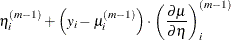
where
 is the variance of Y at
  . Fit an additive model to by using the backfitting algorithm with weights to obtain estimated functions
  ;
;
-
Until: The convergence criterion is satisfied or the deviance fails to decrease. The deviance is an extension to generalized linear models of the RSS; see Goodness of Fit in Chapter 40: The GENMOD Procedure, for a definition.
The GAM procedure uses the following condition as the convergence criterion for local scoring:
![\[ \frac{\sum _{i=1}^ n w_ i \sum _{j=1}^{p} \left(s^{(m-1)}_ j(\mb {X}_{ij}) - s^{(m)}_ j(\mb {X}_{ij})\right)^2}{\sum _{i=1}^ n w_ i \left(1+\sum _{j=1}^{p} \left(s^{(m-1)}_ j(\mb {X}_{ij})\right)^2\right)} \le \epsilon ^{s} \]](images/statug_gam0093.png) |
where ![]() by default; you can change this with the EPSSCORE= option in the MODEL statement.
by default; you can change this with the EPSSCORE= option in the MODEL statement.
The estimating procedure for generalized additive models consists of two loops. Inside each step of the local scoring algorithm (outer loop), a weighted backfitting algorithm (inner loop) is used until convergence or until the RSS fails to decrease. Then, based on the estimates from this weighted backfitting algorithm, a new set of weights is calculated and the next iteration of the scoring algorithm starts. The scoring algorithm stops when the convergence criterion is satisfied or the deviance of the estimates stops decreasing.