The GAM Procedure
- Overview
- Getting Started
-
Syntax

-
DetailsMissing ValuesNonparametric RegressionAdditive Models and Generalized Additive ModelsForms of Additive ModelsEstimates from PROC GAMBackfitting and Local Scoring AlgorithmsSmoothersSelection of Smoothing ParametersConfidence Intervals for SmoothersDistribution Family and Canonical LinkDispersion ParameterComputational ResourcesODS Table NamesODS Graphics
-
Examples
- References
Example 39.3 Comparing PROC GAM with PROC LOESS
In an analysis of simulated data from a hypothetical chemistry experiment, additive nonparametric regression performed by PROC GAM is compared to the unrestricted multidimensional procedure of PROC LOESS.
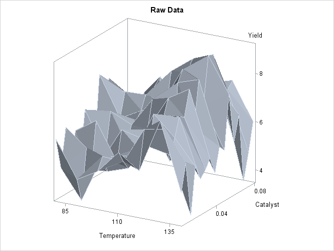
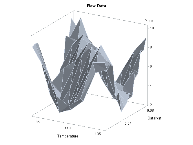
In each repetition of the experiment, a catalyst is added to a chemical solution, thereby inducing synthesis of a new material. The data are measurements of the temperature of the solution, the amount of catalyst added, and the yield of the chemical reaction. The following statements read and plots the raw data.
data ExperimentA;
   format Temperature f4.0 Catalyst f6.3 Yield f8.3;
   input Temperature Catalyst Yield @@;
   datalines;
80  0.005 6.039  80 0.010 4.719  80 0.015 6.301
80  0.020 4.558  80 0.025 5.917  80 0.030 4.365
80  0.035 6.540  80 0.040 5.063  80 0.045 4.668
80  0.050 7.641  80 0.055 6.736  80 0.060 7.255
80  0.065 5.515  80 0.070 5.260  80 0.075 4.813
80  0.080 4.465  90 0.005 4.540  90 0.010 3.553
90  0.015 5.611  90 0.020 4.586  90 0.025 6.503
90  0.030 4.671  90 0.035 4.919  90 0.040 6.536
90  0.045 4.799  90 0.050 6.002  90 0.055 6.988
90  0.060 6.206  90 0.065 5.193  90 0.070 5.783
90  0.075 6.482  90 0.080 5.222 100 0.005 5.042
100 0.010 5.551 100 0.015 4.804 100 0.020 5.313
100 0.025 4.957 100 0.030 6.177 100 0.035 5.433
100 0.040 6.139 100 0.045 6.217 100 0.050 6.498
100 0.055 7.037 100 0.060 5.589 100 0.065 5.593
100 0.070 7.438 100 0.075 4.794 100 0.080 3.692
110 0.005 6.005 110 0.010 5.493 110 0.015 5.107
110 0.020 5.511 110 0.025 5.692 110 0.030 5.969
110 0.035 6.244 110 0.040 7.364 110 0.045 6.412
110 0.050 6.928 110 0.055 6.814 110 0.060 8.071
110 0.065 6.038 110 0.070 6.295 110 0.075 4.308
110 0.080 7.020 120 0.005 5.409 120 0.010 7.009
120 0.015 6.160 120 0.020 7.408 120 0.025 7.123
120 0.030 7.009 120 0.035 7.708 120 0.040 5.278
120 0.045 8.111 120 0.050 8.547 120 0.055 8.279
120 0.060 8.736 120 0.065 6.988 120 0.070 6.283
120 0.075 7.367 120 0.080 6.579 130 0.005 7.629
130 0.010 7.171 130 0.015 5.997 130 0.020 6.587
130 0.025 7.335 130 0.030 7.209 130 0.035 8.259
130 0.040 6.530 130 0.045 8.400 130 0.050 7.218
130 0.055 9.167 130 0.060 9.082 130 0.065 7.680
130 0.070 7.139 130 0.075 7.275 130 0.080 7.544
140 0.005 4.860 140 0.010 5.932 140 0.015 3.685
140 0.020 5.581 140 0.025 4.935 140 0.030 5.197
140 0.035 5.559 140 0.040 4.836 140 0.045 5.795
140 0.050 5.524 140 0.055 7.736 140 0.060 5.628
140 0.065 6.644 140 0.070 3.785 140 0.075 4.853
140 0.080 6.006
;
proc sort data=ExperimentA;
   by Temperature Catalyst;
run;

proc template;
   define statgraph surface;
      dynamic _X _Y _Z _T;
      begingraph;
         entrytitle _T;
         layout overlay3d/
            xaxisopts=(linearopts=(tickvaluesequence=
                       (start=85 end=135 increment=25)))
            yaxisopts=(linearopts=(tickvaluesequence=
                       (start=0 end=0.08 increment=0.04)))
            rotate=30 cube=false;
         surfaceplotparm x=_X y=_Y z=_Z;
         endlayout;
      endgraph;
   end;
run;

ods graphics on;
proc sgrender data=ExperimentA template=surface;
   dynamic _X='Temperature' _Y='Catalyst' _Z='Yield' _T='Raw Data';
run;
The plot is displayed in Output 39.3.1. A surface fitted to the plot of Output 39.3.1 by PROC LOESS will be of a very general (and flexible) type, since the procedure requires only weak assumptions about the structure of the dependencies among the data. PROC GAM, on the other hand, makes stronger structural assumptions by restricting the fitted surface to an additive form. These differences will be demonstrated in this example.
Output 39.3.1: Surface Plot of Yield by Temperature and Amount of Catalyst
The following statements request that both PROC LOESS and PROC GAM fit surfaces to the data:
ods output ScoreResults=PredLOESS;
proc loess data=ExperimentA;
   model Yield = Temperature Catalyst
                 / scale=sd select=gcv degree=2;
   score;
run;

proc gam data=PredLoess;
   model Yield = loess(Temperature) loess(Catalyst) / method=gcv;
   output out=PredGAM p=Gam_p_;
run;
In both cases the smoothing parameter was chosen as the value that minimizes GCV. This is performed automatically by PROC LOESS and PROC GAM.
The following statements generate plots of the predicted yields, which are displayed in Output 39.3.2:
proc template;
   define statgraph surface1;
      begingraph;
         entrytitle "Fitted Surface";
         layout lattice/columns=2;
            layout
            overlay3d/xaxisopts=(linearopts=(tickvaluesequence=
                                (start=85 end=135 increment=25)))
                     yaxisopts=(linearopts=(tickvaluesequence=
                                (start=0 end=0.08 increment=0.04)))
                     zaxisopts=(label="P_Yield")
                     rotate=30 cube=0;
               entry "PROC LOESS"/location=outside valign=top
                                  textattrs=graphlabeltext;
               surfaceplotparm x=Temperature y=Catalyst z=p_Yield;
            endlayout;
            layout
            overlay3d/xaxisopts=(linearopts=(tickvaluesequence=
                                (start=85 end=135 increment=25)))
                     yaxisopts=(linearopts=(tickvaluesequence=
                                (start=0 end=0.08 increment=0.04)))
                     rotate=30 cube=0
                     zaxisopts=(label="P_Yield")
                     rotate=30 cube=0;
               entry "PROC GAM"/location=outside valign=top
                                textattrs=graphlabeltext;
               surfaceplotparm x=Temperature y=Catalyst z=Gam_p_Yield;
            endlayout;
         endlayout;
      endgraph;
   end;
run;

proc sgrender data=PredGAM template=surface1;
run;
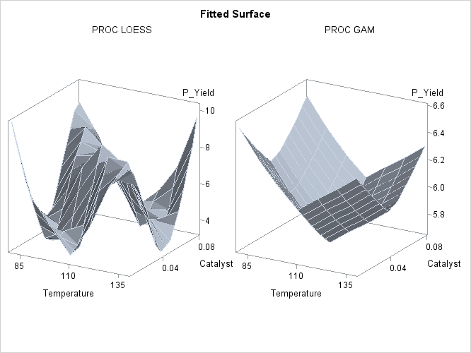
Output 39.3.2: Fitted Regression Surfaces
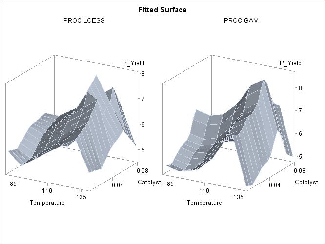
Though both PROC LOESS and PROC GAM use the statistical technique loess, it is apparent from Output 39.3.2 that the manner in which it is applied is very different. By smoothing out the data in local neighborhoods, PROC LOESS essentially fits a surface to the data in pieces, one neighborhood at a time. The local regions are treated independently, so separate areas of the fitted surface are only weakly related. PROC GAM imposes additive structure, requiring that cross sections of the fitted surface always have the same shape and thereby relating regions that have a common value of the same individual regressor variable. Under that restriction, the loess technique need not be applied to the entire multidimensional scatter plot, but only to one-dimensional cross sections of the data.
The advantage of using additive model fitting is that its statistical power is directed toward univariate smoothing, and so it is able to discern the finer details of any underlying structure in the data. Regression data can be very sparse when viewed in the context of multidimensional space, even when every individual set of regressor values densely covers its range. This is the familiar curse of dimensionality. Sparse data greatly restrict the effectiveness of nonparametric procedures, but additive model fitting, when appropriate, is one way to overcome this limitation.
To examine these properties, you can use ODS Graphics to generate plots of cross sections of the unrestricted (PROC LOESS)
and additive (PROC GAM) fitted surfaces for the variable Catalyst, as shown in the following statements:
proc template;
   define statgraph projection;
      begingraph;
         entrytitle "Cross Sections of Fitted Surfaces";
         layout lattice/rows=2 columndatarange=unionall
                       columngutter=10;
            columnAxes;
               columnAxis / display=all griddisplay=auto_on;
            endColumnAxes;

            layout overlay/
               xaxisopts=(display=none)
               yaxisopts=(label="LOESS Prediction"
               linearopts=(viewmin=2 viewmax=10));
               seriesplot x=Catalyst y=p_Yield /
                  group=temperature
                  name="Temperature";
            endlayout;

            layout overlay/
               xaxisopts=(display=none)
               yaxisopts=(label="GAM Prediction"
               linearopts=(viewmin=2 viewmax=10));
               seriesplot x=Catalyst y=Gam_p_Yield /
                  group=temperature
                  name="Temperature";
            endlayout;

            columnheaders;
               discreteLegend "Temperature" / title = "Temperature";
            endcolumnheaders;

         endlayout;
      endgraph;
   end;
run;

proc sgrender data=PredGAM template=projection;
run;
The plots are displayed in Output 39.3.3.
Output 39.3.3: Cross Sections of Fitted Regression Surfaces
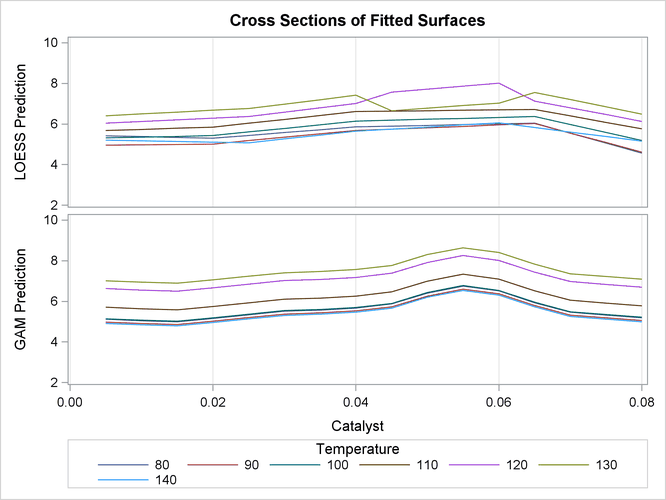
Notice that the cross sections in the top panel (PROC LOESS) of Output 39.3.3 have varying shapes, while every cross section in the bottom panel (PROC GAM) is the same curve shifted vertically. This
illustrates precisely the kind of structural differences that distinguish additive models. A second important comparison to
make between Output 39.3.2 and Output 39.3.3 is the level of detail in the fitted regression surfaces. Cross sections of the PROC LOESS surface are rather flat, but those
of the additive surface have a clear shape. In particular, the ridge near Catalyst=0.055 is only vaguely evident in the PROC LOESS surface, but it is plainly revealed by the additive procedure.
For an example of a situation where unrestricted multidimensional fitting is preferred over additive regression, consider the following simulated data from a similar experiment. The following statements create another SAS data set and plot.
data ExperimentB;
   format Temperature f4.0 Catalyst f6.3 Yield f8.3;
   input Temperature Catalyst Yield @@;
   datalines;
80  0.005  9.115  80 0.010  9.275  80 0.015  9.160
80  0.020  7.065  80 0.025  6.054  80 0.030  4.899
80  0.035  4.504  80 0.040  4.238  80 0.045  3.232
80  0.050  3.135  80 0.055  5.100  80 0.060  4.802
80  0.065  8.218  80 0.070  7.679  80 0.075  9.669
80  0.080  9.071  90 0.005  7.085  90 0.010  6.814
90  0.015  4.009  90 0.020  4.199  90 0.025  3.377
90  0.030  2.141  90 0.035  3.500  90 0.040  5.967
90  0.045  5.268  90 0.050  6.238  90 0.055  7.847
90  0.060  7.992  90 0.065  7.904  90 0.070 10.184
90  0.075  7.914  90 0.080  6.842 100 0.005  4.497
100 0.010  2.565 100 0.015  2.637 100 0.020  2.436
100 0.025  2.525 100 0.030  4.474 100 0.035  6.238
100 0.040  7.029 100 0.045  8.183 100 0.050  8.939
100 0.055  9.283 100 0.060  8.246 100 0.065  6.927
100 0.070  7.062 100 0.075  5.615 100 0.080  4.687
110 0.005  3.706 110 0.010  3.154 110 0.015  3.726
110 0.020  4.634 110 0.025  5.970 110 0.030  8.219
110 0.035  8.590 110 0.040  9.097 110 0.045  7.887
110 0.050  8.480 110 0.055  6.818 110 0.060  7.666
110 0.065  4.375 110 0.070  3.994 110 0.075  3.630
110 0.080  2.685 120 0.005  4.697 120 0.010  4.268
120 0.015  6.507 120 0.020  7.747 120 0.025  9.412
120 0.030  8.761 120 0.035  8.997 120 0.040  7.538
120 0.045  7.003 120 0.050  6.010 120 0.055  3.886
120 0.060  4.897 120 0.065  2.562 120 0.070  2.714
120 0.075  3.141 120 0.080  5.081 130 0.005  8.729
130 0.010  7.460 130 0.015  9.549 130 0.020 10.049
130 0.025  8.131 130 0.030  7.553 130 0.035  6.191
130 0.040  6.272 130 0.045  4.649 130 0.050  3.884
130 0.055  2.522 130 0.060  4.366 130 0.065  3.272
130 0.070  4.906 130 0.075  6.538 130 0.080  7.380
140 0.005  8.991 140 0.010  8.029 140 0.015  8.417
140 0.020  8.049 140 0.025  4.608 140 0.030  5.025
140 0.035  2.795 140 0.040  3.123 140 0.045  3.407
140 0.050  4.183 140 0.055  3.750 140 0.060  6.316
140 0.065  5.799 140 0.070  7.992 140 0.075  7.835
140 0.080  8.985
;
proc sort data=ExperimentB;
   by Temperature Catalyst;
run;

proc sgrender data=ExperimentB template=surface;
   dynamic _X='Temperature' _Y='Catalyst' _Z='Yield' _T='Raw Data';
run;
A plot of the raw data is displayed in Output 39.3.4.
Output 39.3.4: Raw Data from Experiment B
Though the surface displayed in Output 39.3.4 is quite jagged, a distinct feature of the plot is a large ridge that runs diagonally across its surface. One would expect that the ridge would appear in the fitted regression surface of an appropriate nonparametric procedure. Nevertheless, between PROC LOESS and PROC GAM, only PROC LOESS is able to capture this significant feature.
The SAS program for fitting the new data is essentially the same as that for the data set from the first experiment and produces
output data set PredGAMb for this experiment. As in Output 39.3.2, multivariate and additive fitted surfaces for these data are displayed in Output 39.3.5.
Output 39.3.5: Fitted Regression Surfaces
It is clear from Output 39.3.5 that the results of PROC LOESS and PROC GAM are completely different. While the plot in the left panel resembles the raw data plot in Output 39.3.4, the plot in the right panel is essentially featureless.
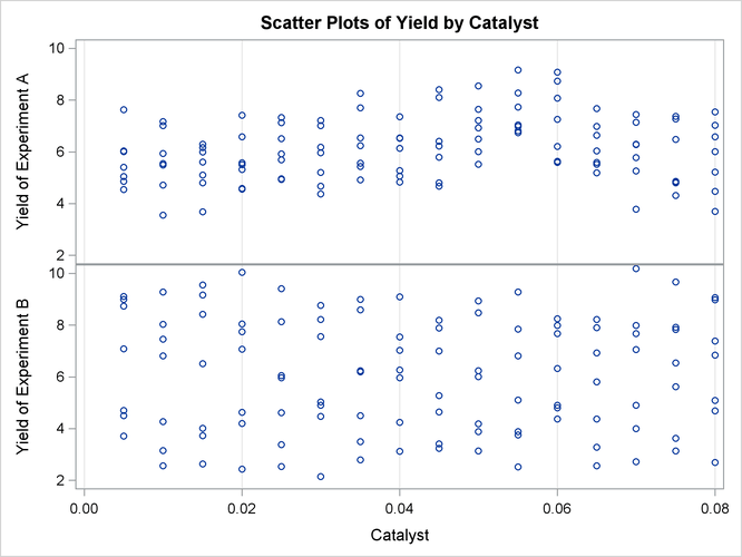
To understand what is happening, compare the scatter plots of Yield by Catalyst for the two data sets in this example. These are generated by the following statements and displayed in Output 39.3.6.
data PredGAM;
   set PredGAM;
   rename Yield=Yield_a;
run;

data PredGAMb;
   set PredGAMb;
   set PredGAM(keep=Yield_a);
run;

proc template;
   define statgraph scatter2;
      dynamic _X _Y1 _Y2;
      begingraph;
         entrytitle "Scatter Plots of Yield by Catalyst";
         layout lattice/rows=2 columndatarange=unionall
                        rowdatarange=unionall
                        columngutter=15;
            columnAxes;
               columnAxis / display=all griddisplay=auto_on;
            endColumnAxes;

            layout overlay/
               xaxisopts=(display=none)
               yaxisopts=(label="Yield of Experiment A"
               linearopts=(viewmin=2 viewmax=10));
               scatterplot x=_X y=_Y1;
            endlayout;

            layout overlay/
               xaxisopts=(display=none)
               yaxisopts=(label="Yield of Experiment B"
               linearopts=(viewmin=2 viewmax=10));
               scatterplot x=_X y=_Y2;
            endlayout;

         endlayout;
      endgraph;
   end;
run;

proc sgrender data=PredGAMb template=scatter2;
   dynamic _X='Catalyst' _Y1='Yield_a' _Y2='Yield';
run;

ods graphics off;
The top panel of Output 39.3.6 hints at the same kind of structure exhibited in the fitted cross sections of Output 39.3.3. In PROC GAM, the additive model component corresponding to Catalyst is fit to a similar scatter plot, with the partial residuals computed in the backfitting algorithm, so it is able to capture
the trend seen here. In contrast, when the second data set is viewed from the perspective of Output 39.3.6, the diagonal ridge apparent in Output 39.3.4 is washed out, and no clear structure shows up in the scatter plot. As a result, the additive model fit produced by PROC
GAM is relatively featureless.
Output 39.3.6: Scatter Plots of Yield by Catalyst