The FASTCLUS Procedure

Example 36.1 Fisher’s Iris Data
The iris data published by Fisher (1936) have been widely used for examples in discriminant analysis and cluster analysis. The sepal length, sepal width, petal length, and petal width are measured in millimeters on 50 iris specimens from each of three species, Iris setosa, I. versicolor, and I. virginica. Mezzich and Solomon (1980) discuss a variety of cluster analyses of the iris data.
In this example, the FASTCLUS procedure is used to find two and then three clusters. In the following code, an output data set is created, and PROC FREQ is invoked to compare the clusters with the species classification. See Output 36.1.1 and Output 36.1.2 for these results.
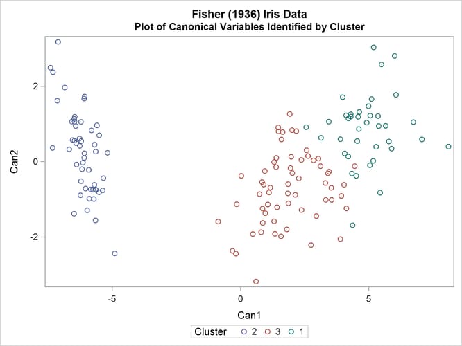
For three clusters, you can use the CANDISC procedure to compute canonical variables for plotting the clusters. See Output 36.1.3 and Output 36.1.4 for the results.
title 'Fisher (1936) Iris Data';
proc fastclus data=sashelp.iris maxc=2 maxiter=10 out=clus;
   var SepalLength SepalWidth PetalLength PetalWidth;
run;

proc freq;
   tables cluster*species;
run;

proc fastclus data=sashelp.iris maxc=3 maxiter=10 out=clus;
   var SepalLength SepalWidth PetalLength PetalWidth;
run;

proc freq;
   tables cluster*Species;
run;

proc candisc anova out=can;
   class cluster;
   var SepalLength SepalWidth PetalLength PetalWidth;
   title2 'Canonical Discriminant Analysis of Iris Clusters';
run;

proc sgplot data=Can;
   scatter y=Can2 x=Can1 / group=Cluster;
   title2 'Plot of Canonical Variables Identified by Cluster';
run;
Output 36.1.1: Fisher’s Iris Data: PROC FASTCLUS with MAXC=2 and PROC FREQ
| Fisher (1936) Iris Data |
| Initial Seeds | ||||
|---|---|---|---|---|
| Cluster | SepalLength | SepalWidth | PetalLength | PetalWidth |
| 1 | 77.00000000 | 26.00000000 | 69.00000000 | 23.00000000 |
| 2 | 45.00000000 | 23.00000000 | 13.00000000 | 3.00000000 |
| Minimum Distance Between Initial Seeds = | 67.59438 |
|---|
| Iteration History | |||
|---|---|---|---|
| Iteration | Criterion | Relative Change in Cluster Seeds |
|
| 1 | 2 | ||
| 1 | 11.0045 | 0.3169 | 0.2164 |
| 2 | 5.6161 | 0.0379 | 0.0791 |
| 3 | 5.1042 | 0.0133 | 0.0306 |
| 4 | 5.0417 | 0.00348 | 0.00679 |
| Convergence criterion is satisfied. |
| Criterion Based on Final Seeds = | 5.0390 |
|---|
| Cluster Summary | ||||||
|---|---|---|---|---|---|---|
| Cluster | Frequency | RMS Std Deviation | Maximum Distance from Seed to Observation |
Radius Exceeded |
Nearest Cluster | Distance Between Cluster Centroids |
| 1 | 97 | 5.6779 | 24.8448 | 2 | 39.2879 | |
| 2 | 53 | 3.7050 | 21.6197 | 1 | 39.2879 | |
| Statistics for Variables | ||||
|---|---|---|---|---|
| Variable | Total STD | Within STD | R-Square | RSQ/(1-RSQ) |
| SepalLength | 8.28066 | 5.49313 | 0.562896 | 1.287784 |
| SepalWidth | 4.35866 | 3.70393 | 0.282710 | 0.394137 |
| PetalLength | 17.65298 | 6.80331 | 0.852470 | 5.778291 |
| PetalWidth | 7.62238 | 3.57200 | 0.781868 | 3.584390 |
| OVER-ALL | 10.69224 | 5.07291 | 0.776410 | 3.472463 |
| Pseudo F Statistic = | 513.92 |
|---|
| Approximate Expected Over-All R-Squared = | 0.51539 |
|---|
| Cubic Clustering Criterion = | 14.806 |
|---|
| Cluster Means | ||||
|---|---|---|---|---|
| Cluster | SepalLength | SepalWidth | PetalLength | PetalWidth |
| 1 | 63.01030928 | 28.86597938 | 49.58762887 | 16.95876289 |
| 2 | 50.05660377 | 33.69811321 | 15.60377358 | 2.90566038 |
| Cluster Standard Deviations | ||||
|---|---|---|---|---|
| Cluster | SepalLength | SepalWidth | PetalLength | PetalWidth |
| 1 | 6.336887455 | 3.267991438 | 7.800577673 | 4.155612484 |
| 2 | 3.427350930 | 4.396611045 | 4.404279486 | 2.105525249 |
| Fisher (1936) Iris Data |
|
|
||||||||||||||||||||||||||||||||||||||||||||||||||||||||||||||||||||||||||
Output 36.1.2: Fisher’s Iris Data: PROC FASTCLUS with MAXC=3 and PROC FREQ
| Fisher (1936) Iris Data |
| Initial Seeds | ||||
|---|---|---|---|---|
| Cluster | SepalLength | SepalWidth | PetalLength | PetalWidth |
| 1 | 77.00000000 | 38.00000000 | 67.00000000 | 22.00000000 |
| 2 | 57.00000000 | 44.00000000 | 15.00000000 | 4.00000000 |
| 3 | 49.00000000 | 25.00000000 | 45.00000000 | 17.00000000 |
| Minimum Distance Between Initial Seeds = | 38.23611 |
|---|
| Iteration History | ||||
|---|---|---|---|---|
| Iteration | Criterion | Relative Change in Cluster Seeds | ||
| 1 | 2 | 3 | ||
| 1 | 7.0151 | 0.3205 | 0.3151 | 0.2985 |
| 2 | 3.7097 | 0.0459 | 0 | 0.0317 |
| 3 | 3.6427 | 0.0182 | 0 | 0.0124 |
| Convergence criterion is satisfied. |
| Criterion Based on Final Seeds = | 3.6289 |
|---|
| Cluster Summary | ||||||
|---|---|---|---|---|---|---|
| Cluster | Frequency | RMS Std Deviation | Maximum Distance from Seed to Observation |
Radius Exceeded |
Nearest Cluster | Distance Between Cluster Centroids |
| 1 | 38 | 4.0168 | 14.9736 | 3 | 17.9718 | |
| 2 | 50 | 2.7803 | 12.4803 | 3 | 33.5693 | |
| 3 | 62 | 4.0398 | 16.9272 | 1 | 17.9718 | |
| Statistics for Variables | ||||
|---|---|---|---|---|
| Variable | Total STD | Within STD | R-Square | RSQ/(1-RSQ) |
| SepalLength | 8.28066 | 4.39488 | 0.722096 | 2.598359 |
| SepalWidth | 4.35866 | 3.24816 | 0.452102 | 0.825156 |
| PetalLength | 17.65298 | 4.21431 | 0.943773 | 16.784895 |
| PetalWidth | 7.62238 | 2.45244 | 0.897872 | 8.791618 |
| OVER-ALL | 10.69224 | 3.66198 | 0.884275 | 7.641194 |
| Pseudo F Statistic = | 561.63 |
|---|
| Approximate Expected Over-All R-Squared = | 0.62728 |
|---|
| Cubic Clustering Criterion = | 25.021 |
|---|
| Cluster Means | ||||
|---|---|---|---|---|
| Cluster | SepalLength | SepalWidth | PetalLength | PetalWidth |
| 1 | 68.50000000 | 30.73684211 | 57.42105263 | 20.71052632 |
| 2 | 50.06000000 | 34.28000000 | 14.62000000 | 2.46000000 |
| 3 | 59.01612903 | 27.48387097 | 43.93548387 | 14.33870968 |
| Cluster Standard Deviations | ||||
|---|---|---|---|---|
| Cluster | SepalLength | SepalWidth | PetalLength | PetalWidth |
| 1 | 4.941550255 | 2.900924461 | 4.885895746 | 2.798724562 |
| 2 | 3.524896872 | 3.790643691 | 1.736639965 | 1.053855894 |
| 3 | 4.664100551 | 2.962840548 | 5.088949673 | 2.974997167 |
| Fisher (1936) Iris Data |
|
|
|||||||||||||||||||||||||||||||||||||||||||||||||||||||||||||||||||||||||||||||||||||||||||||||
Output 36.1.3: Fisher’s Iris Data using PROC CANDISC
| Fisher (1936) Iris Data |
| Canonical Discriminant Analysis of Iris Clusters |
| Total Sample Size | 150 | DF Total | 149 |
|---|---|---|---|
| Variables | 4 | DF Within Classes | 147 |
| Classes | 3 | DF Between Classes | 2 |
| Number of Observations Read | 150 |
|---|---|
| Number of Observations Used | 150 |
| Class Level Information | ||||
|---|---|---|---|---|
| CLUSTER | Variable Name |
Frequency | Weight | Proportion |
| 1 | _1 | 38 | 38.0000 | 0.253333 |
| 2 | _2 | 50 | 50.0000 | 0.333333 |
| 3 | _3 | 62 | 62.0000 | 0.413333 |
| Fisher (1936) Iris Data |
| Canonical Discriminant Analysis of Iris Clusters |
| Univariate Test Statistics | ||||||||
|---|---|---|---|---|---|---|---|---|
| F Statistics, Num DF=2, Den DF=147 | ||||||||
| Variable | Label | Total Standard Deviation |
Pooled Standard Deviation |
Between Standard Deviation |
R-Square | R-Square / (1-RSq) |
F Value | Pr > F |
| SepalLength | Sepal Length (mm) | 8.2807 | 4.3949 | 8.5893 | 0.7221 | 2.5984 | 190.98 | <.0001 |
| SepalWidth | Sepal Width (mm) | 4.3587 | 3.2482 | 3.5774 | 0.4521 | 0.8252 | 60.65 | <.0001 |
| PetalLength | Petal Length (mm) | 17.6530 | 4.2143 | 20.9336 | 0.9438 | 16.7849 | 1233.69 | <.0001 |
| PetalWidth | Petal Width (mm) | 7.6224 | 2.4524 | 8.8164 | 0.8979 | 8.7916 | 646.18 | <.0001 |
| Average R-Square | |
|---|---|
| Unweighted | 0.7539604 |
| Weighted by Variance | 0.8842753 |
| Multivariate Statistics and F Approximations | |||||
|---|---|---|---|---|---|
| S=2 M=0.5 N=71 | |||||
| Statistic | Value | F Value | Num DF | Den DF | Pr > F |
| Wilks' Lambda | 0.03222337 | 164.55 | 8 | 288 | <.0001 |
| Pillai's Trace | 1.25669612 | 61.29 | 8 | 290 | <.0001 |
| Hotelling-Lawley Trace | 21.06722883 | 377.66 | 8 | 203.4 | <.0001 |
| Roy's Greatest Root | 20.63266809 | 747.93 | 4 | 145 | <.0001 |
| NOTE: F Statistic for Roy's Greatest Root is an upper bound. | |||||
| NOTE: F Statistic for Wilks' Lambda is exact. | |||||
| Fisher (1936) Iris Data |
| Canonical Discriminant Analysis of Iris Clusters |
| Canonical Correlation |
Adjusted Canonical Correlation |
Approximate Standard Error |
Squared Canonical Correlation |
Eigenvalues of Inv(E)*H = CanRsq/(1-CanRsq) |
Test of H0: The canonical correlations in the current row and all that follow are zero | ||||||||
|---|---|---|---|---|---|---|---|---|---|---|---|---|---|
| Eigenvalue | Difference | Proportion | Cumulative | Likelihood Ratio |
Approximate F Value |
Num DF | Den DF | Pr > F | |||||
| 1 | 0.976613 | 0.976123 | 0.003787 | 0.953774 | 20.6327 | 20.1981 | 0.9794 | 0.9794 | 0.03222337 | 164.55 | 8 | 288 | <.0001 |
| 2 | 0.550384 | 0.543354 | 0.057107 | 0.302923 | 0.4346 | 0.0206 | 1.0000 | 0.69707749 | 21.00 | 3 | 145 | <.0001 | |
| Fisher (1936) Iris Data |
| Canonical Discriminant Analysis of Iris Clusters |
| Total Canonical Structure | |||
|---|---|---|---|
| Variable | Label | Can1 | Can2 |
| SepalLength | Sepal Length (mm) | 0.831965 | 0.452137 |
| SepalWidth | Sepal Width (mm) | -0.515082 | 0.810630 |
| PetalLength | Petal Length (mm) | 0.993520 | 0.087514 |
| PetalWidth | Petal Width (mm) | 0.966325 | 0.154745 |
| Between Canonical Structure | |||
|---|---|---|---|
| Variable | Label | Can1 | Can2 |
| SepalLength | Sepal Length (mm) | 0.956160 | 0.292846 |
| SepalWidth | Sepal Width (mm) | -0.748136 | 0.663545 |
| PetalLength | Petal Length (mm) | 0.998770 | 0.049580 |
| PetalWidth | Petal Width (mm) | 0.995952 | 0.089883 |
| Pooled Within Canonical Structure | |||
|---|---|---|---|
| Variable | Label | Can1 | Can2 |
| SepalLength | Sepal Length (mm) | 0.339314 | 0.716082 |
| SepalWidth | Sepal Width (mm) | -0.149614 | 0.914351 |
| PetalLength | Petal Length (mm) | 0.900839 | 0.308136 |
| PetalWidth | Petal Width (mm) | 0.650123 | 0.404282 |
| Fisher (1936) Iris Data |
| Canonical Discriminant Analysis of Iris Clusters |
| Total-Sample Standardized Canonical Coefficients | |||
|---|---|---|---|
| Variable | Label | Can1 | Can2 |
| SepalLength | Sepal Length (mm) | 0.047747341 | 1.021487262 |
| SepalWidth | Sepal Width (mm) | -0.577569244 | 0.864455153 |
| PetalLength | Petal Length (mm) | 3.341309573 | -1.283043758 |
| PetalWidth | Petal Width (mm) | 0.996451144 | 0.900476563 |
| Pooled Within-Class Standardized Canonical Coefficients | |||
|---|---|---|---|
| Variable | Label | Can1 | Can2 |
| SepalLength | Sepal Length (mm) | 0.0253414487 | 0.5421446856 |
| SepalWidth | Sepal Width (mm) | -.4304161258 | 0.6442092294 |
| PetalLength | Petal Length (mm) | 0.7976741592 | -.3063023132 |
| PetalWidth | Petal Width (mm) | 0.3205998034 | 0.2897207865 |
| Raw Canonical Coefficients | |||
|---|---|---|---|
| Variable | Label | Can1 | Can2 |
| SepalLength | Sepal Length (mm) | 0.0057661265 | 0.1233581748 |
| SepalWidth | Sepal Width (mm) | -.1325106494 | 0.1983303556 |
| PetalLength | Petal Length (mm) | 0.1892773419 | -.0726814163 |
| PetalWidth | Petal Width (mm) | 0.1307270927 | 0.1181359305 |
| Class Means on Canonical Variables | ||
|---|---|---|
| CLUSTER | Can1 | Can2 |
| 1 | 4.931414018 | 0.861972277 |
| 2 | -6.131527227 | 0.244761516 |
| 3 | 1.922300462 | -0.725693908 |
Output 36.1.4: Plot of Fisher’s Iris Data using PROC CANDISC