The QUANTREG Procedure

| Analysis of Fish-Habitat Relationships |
Quantile regression is used extensively in ecological studies (Cade and Noon 2003). Recently, Dunham, Cade, and Terrell (2002) applied quantile regression to analyze fish-habitat relationships for Lahontan cutthroat trout in 13 streams of the eastern Lahontan basin, which covers most of northern Nevada and parts of southern Oregon. The density of trout (number of trout per meter) was measured by sampling stream sites from 1993 to 1999. The width-to-depth ratio of the stream site was determined as a measure of stream habitat.
The goal of this study was to explore the relationship between the conditional quantiles of trout density and the width-to-depth ratio. The scatter plot of the data in Figure 75.1 indicates a nonlinear relationship, and so it is reasonable to fit regression models for the conditional quantiles of the log of density. Since regression quantiles are equivariant under any monotonic (linear or nonlinear) transformation (Koenker and Hallock 2001), the exponential transformation converts the conditional quantiles to the original density scale.
The data set trout, which follows, includes the average numbers of Lahontan cutthroat trout per meter of stream (Density), the logarithm of Density (LnDensity), and the width-to-depth ratios (WDRatio) for 71 samples.
data trout;
  input Density WDRatio LnDensity @@;
  datalines;
 0.38732     8.6819    -0.94850    1.16956    10.5102     0.15662
 0.42025    10.7636    -0.86690    0.50059    12.7884    -0.69197
 0.74235    12.9266    -0.29793    0.40385    14.4884    -0.90672
 0.35245    15.2476    -1.04284    0.11499    16.6495    -2.16289
 0.18290    16.7188    -1.69881    0.06619    16.7859    -2.71523

   ... more lines ...

 0.25125    54.6916    -1.38129
 ;
The following statements use the QUANTREG procedure to fit a simple linear model for the 50th and 90th percentiles of LnDensity:
ods graphics on;

proc quantreg data=trout alpha=0.1 ci=resampling;
   model LnDensity = WDRatio / quantile=0.5 0.9
                               CovB seed=1268;
   test WDRatio / wald lr;
run;
The MODEL statement specifies a simple linear regression model with LnDensity as the response variable Y and WDRatio as the covariate X. The QUANTILE= option requests that the regression quantile function 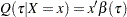 be estimated by solving
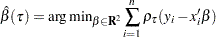 |
where  .
.
By default, the regression coefficients  are estimated with the simplex algorithm, which is explained in the section Simplex Algorithm. The ALPHA= option requests
  confidence limits for the regression parameters, and the option CI=RESAMPLING specifies that the intervals are to be computed with the MCMB resampling method of He and Hu (2002). By specifying the CI=RESAMPLING option, the QUANTREG procedure also computes standard errors, t values, and p-values of regression parameters with the MCMB resampling method. The SEED= option specifies a seed for the resampling method. The COVB option requests covariance matrices for the estimated regression coefficients, and the TEST statement requests tests for the hypothesis that the slope parameter (the coefficient of WDRatio) is zero.
Figure 75.3 displays model information and summary statistics for the variables in the model. The summary statistics include the median and the standardized median absolute deviation (MAD), which are robust measures of univariate location and scale, respectively. See Huber (1981, p. 108) for more details about the standardized MAD.
| Model Information | |
|---|---|
| Data Set | WORK.TROUT |
| Dependent Variable | LnDensity |
| Number of Independent Variables | 1 |
| Number of Observations | 71 |
| Optimization Algorithm | Simplex |
| Method for Confidence Limits | Resampling |
| Summary Statistics | ||||||
|---|---|---|---|---|---|---|
| Variable | Q1 | Median | Q3 | Mean | Standard Deviation |
MAD |
| WDRatio | 22.0917 | 29.4083 | 35.9382 | 29.1752 | 9.9859 | 10.4970 |
| LnDensity | -2.0511 | -1.3813 | -0.8669 | -1.4973 | 0.7682 | 0.8214 |
Figure 75.4 and Figure 75.5 display the parameter estimates, standard errors, 95 confidence limits, t values, and p-values that are computed by the resampling method.
| Parameter Estimates | |||||||
|---|---|---|---|---|---|---|---|
| Parameter | DF | Estimate | Standard Error | 90% Confidence Limits | t Value | Pr > |t| | |
| Intercept | 1 | -0.9811 | 0.3952 | -1.6400 | -0.3222 | -2.48 | 0.0155 |
| WDRatio | 1 | -0.0136 | 0.0123 | -0.0341 | 0.0068 | -1.11 | 0.2705 |
| Parameter Estimates | |||||||
|---|---|---|---|---|---|---|---|
| Parameter | DF | Estimate | Standard Error | 90% Confidence Limits | t Value | Pr > |t| | |
| Intercept | 1 | 0.0576 | 0.2606 | -0.3769 | 0.4921 | 0.22 | 0.8257 |
| WDRatio | 1 | -0.0215 | 0.0075 | -0.0340 | -0.0091 | -2.88 | 0.0053 |
The 90th percentile of trout density can be predicted from the width-to-depth ratio as follows:
 |
This is the upper dashed curve plotted in Figure 75.1. The lower dashed curve for the median can be obtained in a similar fashion.
The covariance matrices for the estimated parameters are shown in Figure 75.6. The resampling method used for the confidence intervals is used to compute these matrices.
| Estimated Covariance Matrix for Quantile = 0.5 |
||
|---|---|---|
| Intercept | WDRatio | |
| Intercept | 0.156191 | -.004653 |
| WDRatio | -.004653 | 0.000151 |
| Estimated Covariance Matrix for Quantile = 0.9 |
||
|---|---|---|
| Intercept | WDRatio | |
| Intercept | 0.067914 | -.001877 |
| WDRatio | -.001877 | 0.000056 |
The tests requested with the TEST statement are shown in Figure 75.7. Both the Wald test and the likelihood ratio test indicate that the coefficient of width-to-depth ratio is significantly different from zero at the 90th percentile, but the deference is not significant at the median.
| Test Results | |||||
|---|---|---|---|---|---|
| Quantile | Test | Test Statistic | DF | Chi-Square | Pr > ChiSq |
| 0.5 | Wald | 1.2339 | 1 | 1.23 | 0.2666 |
| 0.5 | Likelihood Ratio | 1.1467 | 1 | 1.15 | 0.2842 |
| 0.9 | Wald | 8.3031 | 1 | 8.30 | 0.0040 |
| 0.9 | Likelihood Ratio | 9.0529 | 1 | 9.05 | 0.0026 |
In many quantile regression problems it is useful to examine how the estimated regression parameters for each covariate change as a function of  in the interval
  . The following statements use the QUANTREG procedure to request the estimated quantile processes
  for the slope and intercept parameters:
proc quantreg data=trout alpha=0.1 ci=resampling;
   model LnDensity = WDRatio / quantile=process seed=1268
                               plot=quantplot;
run;
The QUANTILE=PROCESS option requests an estimate of the quantile process for each regression parameter. The options ALPHA=0.1 and CI=RESAMPLING specify that 90 confidence bands for the quantile processes are to be computed with the resampling method.
Figure 75.8 displays a portion of the objective function table for the entire quantile process. The objective function is evaluated at 77 values of in the interval . The table also provides predicted values of the conditional quantile function  at the mean for WDRatio, which can be used to estimate the conditional density function.
| Objective Function for Quantile Process |
|||
|---|---|---|---|
| Label | Quantile | Objective Function |
Predicted at Mean |
| t0 | 0.005634 | 0.7044 | -3.2582 |
| t1 | 0.020260 | 2.5331 | -3.0331 |
| t2 | 0.031348 | 3.7421 | -2.9376 |
| t3 | 0.046131 | 5.2538 | -2.7013 |
| . | . | . | . |
| . | . | . | . |
| . | . | . | . |
| t73 | 0.945705 | 4.1433 | -0.4361 |
| t74 | 0.966377 | 2.5858 | -0.4287 |
| t75 | 0.976060 | 1.8512 | -0.4082 |
| t76 | 0.994366 | 0.4356 | -0.4082 |
Figure 75.9 displays a portion of the table of the quantile processes for the estimated parameters and confidence limits.
| Parameter Estimates for Quantile Process | |||
|---|---|---|---|
| Label | Quantile | Intercept | WDRatio |
| . | . | . | . |
| . | . | . | . |
| . | . | . | . |
| t57 | 0.765705 | -0.42205 | -0.01335 |
| lower90 | 0.765705 | -0.91952 | -0.02682 |
| upper90 | 0.765705 | 0.07541 | 0.00012 |
| t58 | 0.786206 | -0.32688 | -0.01592 |
| lower90 | 0.786206 | -0.80883 | -0.02895 |
| upper90 | 0.786206 | 0.15507 | -0.00289 |
| . | . | . | . |
| . | . | . | . |
| . | . | . | . |
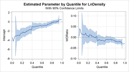
The PLOT=QUANTPLOT option in the MODEL statement, together with ODS Graphics, requests a plot of the estimated quantile processes. The left side of Figure 75.10 displays the process for the intercept, and the right side displays the process for the coefficient of WDRatio.
The process plot for WDRatio shows that the slope parameter changes from positive to negative as the quantile increases, and it changes sign with a sharp drop at the 40th percentile. The 90 confidence bands show that the relationship between LnDensity and WDRatio (expressed by the slope) is not significant below the 78th percentile. This situation can also be seen in Figure 75.9, which shows that 0 falls between the lower and upper confidence limits of the slope parameter for quantiles below 0.78. Since the confidence intervals for the extreme quantiles are not stable due to insufficient data, the confidence band is not displayed outside the interval (0.05, 0.95).