The POWER Procedure

Two-Sample t Test Assuming Equal Variances (TEST=DIFF)

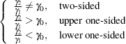
The hypotheses for the two-sample test are

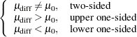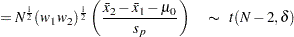
The test assumes normally distributed data and common standard deviation per group, and it requires , , and . The test statistics are

where and are the sample means and is the pooled standard deviation, and

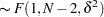
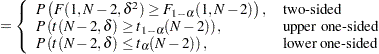
The test is

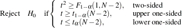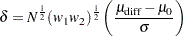
Exact power computations for tests are given in O’Brien and Muller (1993, Section 8.2.1):

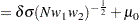
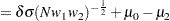
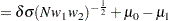
Solutions for , , , , and are obtained by numerically inverting the power equation. Closed-form solutions for other parameters, in terms of , are as follows:

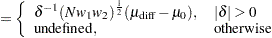
Finally, here is a derivation of the solution for :

Solve the equation for (which requires the quadratic formula). Then determine the range of given :

This implies

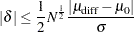Two-Sample Satterthwaite t Test Assuming Unequal Variances (TEST=DIFF_SATT)

The hypotheses for the two-sample Satterthwaite test are

The test assumes normally distributed data and requires , , and . The test statistics are

where and are the sample means and and are the sample standard deviations.

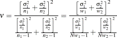
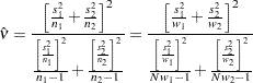
As DiSantostefano and Muller (1995, p. 585) state, the test is based on assuming that under , is distributed as , where is given by Satterthwaite’s approximation (Satterthwaite 1946),

Since is unknown, in practice it must be replaced by an estimate

So the test is

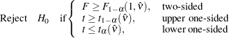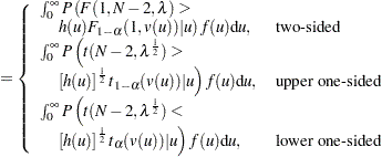
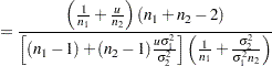
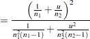
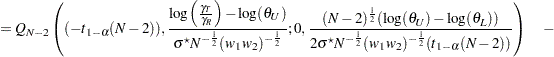
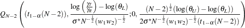
Exact solutions for power for the two-sided and upper one-sided cases are given in Moser, Stevens, and Watts (1989). The lower one-sided case follows easily by using symmetry. The equations are as follows:

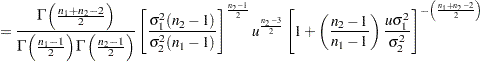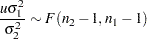
The density is obtained from the fact that

Two-Sample Pooled t Test of Mean Ratio with Lognormal Data (TEST=RATIO)

The lognormal case is handled by reexpressing the analysis equivalently as a normality-based test on the log-transformed data, by using properties of the lognormal distribution as discussed in Johnson, Kotz, and Balakrishnan (1994, Chapter 14). The approaches in the section Two-Sample t Test Assuming Equal Variances (TEST=DIFF) then apply.

In contrast to the usual test on normal data, the hypotheses with lognormal data are defined in terms of geometric means rather than arithmetic means. The test assumes equal coefficients of variation in the two groups.

The hypotheses for the two-sample test with lognormal data are

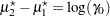
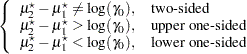
Let , , and be the (arithmetic) means and common standard deviation of the corresponding normal distributions of the log-transformed data. The hypotheses can be rewritten as follows:

where

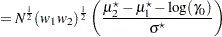
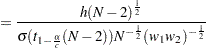
The test assumes lognormally distributed data and requires , , and .

The power is

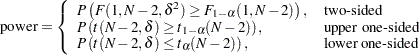where

Additive Equivalence Test for Mean Difference with Normal Data (TEST=EQUIV_DIFF)

The hypotheses for the equivalence test are

The analysis is the two one-sided tests (TOST) procedure of Schuirmann (1987). The test assumes normally distributed data and requires , , and . Phillips (1990) derives an expression for the exact power assuming a balanced design; the results are easily adapted to an unbalanced design:

where is Owen’s Q function, defined in the section Common Notation.

Multiplicative Equivalence Test for Mean Ratio with Lognormal Data (TEST=EQUIV_RATIO)

The lognormal case is handled by reexpressing the analysis equivalently as a normality-based test on the log-transformed data, by using properties of the lognormal distribution as discussed in Johnson, Kotz, and Balakrishnan (1994, Chapter 14). The approaches in the section Additive Equivalence Test for Mean Difference with Normal Data (TEST=EQUIV_DIFF) then apply.

In contrast to the additive equivalence test on normal data, the hypotheses with lognormal data are defined in terms of geometric means rather than arithmetic means.

The hypotheses for the equivalence test are

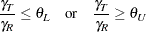The analysis is the two one-sided tests (TOST) procedure of Schuirmann (1987) on the log-transformed data. The test assumes lognormally distributed data and requires , , and . Diletti, Hauschke, and Steinijans (1991) derive an expression for the exact power assuming a crossover design; the results are easily adapted to an unbalanced two-sample design:

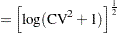
where

is the (assumed common) standard deviation of the normal distribution of the log-transformed data, and is Owen’s Q function, defined in the section Common Notation.

Confidence Interval for Mean Difference (CI=DIFF)

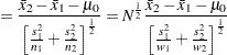
This analysis of precision applies to the standard -based confidence interval:

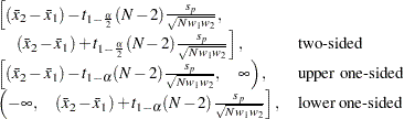where and are the sample means and is the pooled standard deviation. The "half-width" is defined as the distance from the point estimate to a finite endpoint,

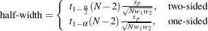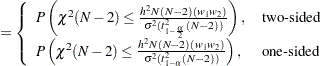
A "valid" conference interval captures the true mean. The exact probability of obtaining at most the target confidence interval half-width , unconditional or conditional on validity, is given by Beal (1989):

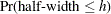where

and is Owen’s Q function, defined in the section Common Notation.

A "quality" confidence interval is both sufficiently narrow (half-width ) and valid: