Testing Covariance Patterns
The most basic use of PROC CALIS is testing covariance patterns. Consider a repeated-measures experiment where individuals are tested for their motor skills at three different time points. No treatments are introduced between these tests. The three test scores are denoted as  ,
,  , and
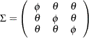
, and  , respectively. These test scores are likely correlated because the same set of individuals has been used. More specifically, the researcher wants to test the following pattern of the population covariance matrix
  :
:
Because there are no treatments between the tests, this pattern assumes that the distribution of motor skills stays more or less the same over time, as represented by the same  for the diagonal elements of . The covariances between the test scores for motor skills also stay the same, as represented by the same
  for all the off-diagonal elements of .
Suppose you summarize your data in a covariance matrix, which is stored in the following SAS data set:
data motor(type=cov);
   input _type_ $ _name_ $ x1 x2 x3;
   datalines;
COV     x1      3.566   1.342   1.114
COV     x2      1.342   4.012   1.056
COV     x3      1.114   1.056   3.776
N        .         36      36      36
;
The diagonal elements are somewhat close to each other but are not the same. The off-diagonal elements are also very close to each other but are not the same. Could these observed differences be due to chance? Given the sample covariance matrix, can you test the hypothesized patterned covariance matrix in the population?
Setting up this patterned covariance model in PROC CALIS is straightforward with the MSTRUCT modeling language:
proc calis data=motor;
   mstruct var  = x1-x3;
   matrix _cov_ = phi
                  theta phi
                  theta theta phi;
run;
In the VAR= option in the MSTRUCT statement, you specify that x1–x3 are the variables in the covariance matrix. Next, you specify the elements of the patterned covariance matrix in the MATRIX statement with the _COV_ keyword. Because the covariance matrix is symmetric, you need to specify only the lower triangular elements in the MATRIX statement. You use phi for the parameters of all diagonal elements and theta for the parameters of all off-diagonal elements. Matrix elements with the same parameter name are implicitly constrained to be equal. Hence, this is the patterned covariance matrix that you want to test. Some output results from PROC CALIS are shown in Figure 17.1.
Figure 17.1
Fit Summary
| 3.7847 |
| 0.5701 |
| 6.6383 |
| [phi] |
|
| 1.1707 |
| 0.5099 |
| 2.2960 |
| [theta] |
|
| 1.1707 |
| 0.5099 |
| 2.2960 |
| [theta] |
|
| 1.1707 |
| 0.5099 |
| 2.2960 |
| [theta] |
|
| 3.7847 |
| 0.5701 |
| 6.6383 |
| [phi] |
|
| 1.1707 |
| 0.5099 |
| 2.2960 |
| [theta] |
|
| 1.1707 |
| 0.5099 |
| 2.2960 |
| [theta] |
|
| 1.1707 |
| 0.5099 |
| 2.2960 |
| [theta] |
|
| 3.7847 |
| 0.5701 |
| 6.6383 |
| [phi] |
|
First, PROC CALIS shows that the chi-square test for the model fit is 0.3656 ( =4,
=4,  =0.9852). Because the chi-square test is not significant, it supports the hypothesized patterned covariance model. Next, PROC CALIS shows the estimates in the covariance matrix under the hypothesized model. The estimates for the diagonal elements are all 3.7847, and the estimates for off-diagonal elements are all 1.1707. Estimates of standard errors and
  values for these covariance and variance parameters are also shown.
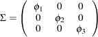
The MSTRUCT modeling language in PROC CALIS enables you to test various kinds of covariance and mean patterns, including matrices with fixed or constrained values. For example, consider a population covariance model in which correlations among the motor test scores are hypothesized to be zero. In other words, the covariance pattern is:
Essentially, this diagonally-patterned covariance model means that the data are randomly and independently generated for x1–x3 under the multivariate normal distribution. Only the variances of the variables are parameters in the model, and the variables are not correlated at all.
You can use the MSTRUCT modeling language of PROC CALIS to fit this diagonally-patterned covariance matrix to the data for motor skills, as shown in the following statements:
proc calis data=motor;
   mstruct var  = x1-x3;
   matrix _cov_ = phi1
                     0.   phi2
                     0.      0.    phi3;
run;
Some of the output is shown in Figure 17.2.
Figure 17.2
Fit Summary: Testing Uncorrelatedness
| 3.5660 |
| 0.8524 |
| 4.1833 |
| [phi1] |
|
|
|
|
| 4.0120 |
| 0.9591 |
| 4.1833 |
| [phi2] |
|
|
|
|
| 3.7760 |
| 0.9026 |
| 4.1833 |
| [phi3] |
|
PROC CALIS shows that the chi-square test for the model fit is 9.2939 (=3, =0.0256). Because the chi-square test is significant, it does not support the patterned covariance model that postulates zero correlations among the variables. This conclusion is consistent with what is already known—the motor test scores should be somewhat correlated because they are measurements over time for the same group of individuals.
The output also shows the estimates of variances under the model. Each diagonal element of the covariance matrix has a distinct estimate because different parameters have been hypothesized under the patterned covariance model.
Testing Built-In Covariance Patterns in PROC CALIS
Some covariance patterns are well-known in multivariate statistics. For example, testing the diagonal pattern for a covariance matrix in the preceding section is a test of uncorrelatedness between the observed variables. Under the multivariate normal assumption, this test is also a test of independence between the observed variables. This test of independence is routinely applied in maximum likelihood factor analysis for testing the zero common factor hypothesis for the observed variables. For testing such a well-known covariance pattern, PROC CALIS provides an efficient way of specifying a model. With the COVPATTERN= option, you can invoke the built-in covariance patterns in PROC CALIS without the MSTRUCT model specifications, which could become laborious when the number of variables are large.
For example, to test the diagonal pattern (uncorrelatedness) of the motor skills, you can simply use the following specification:
proc calis data=motor covpattern=uncorr;
run;
The COVPATTERN=UNCORR option in the PROC CALIS statement invokes the diagonally patterned covariance matrix for the motor skills. PROC CALIS then generates the appropriate free parameters for this built-in covariance pattern. As a result, the MATRIX statement is not needed for specifying the free parameters, as it is if you use explicit MSTRUCT model specifications. Some of the output for using the COVPATTERN= option is shown in Figure 17.3.
Figure 17.3
Fit Summary: Testing Uncorrelatedness with the COVPATTERN= Option
| 3.5660 |
| 0.8524 |
| 4.1833 |
| [_varparm_1] |
|
|
|
|
| 4.0120 |
| 0.9591 |
| 4.1833 |
| [_varparm_2] |
|
|
|
|
| 3.7760 |
| 0.9026 |
| 4.1833 |
| [_varparm_3] |
|
In the second table of
Figure 17.3, the estimates of variances and their standard errors are the same as those shown in
Figure 17.2. The only difference is that the parameter names (for example,
_varparm_1) for the variances in
Figure 17.3 are generated by PROC CALIS, instead of being specified as those in
Figure 17.2.
However, the current chi-square test for the model fit is 8.8071 (=3, =0.0320), which is different from that in Figure 17.2 for testing the same covariance pattern. The reason is that the chi-square correction due to Bartlett (1950) has been applied automatically to the current built-in covariance pattern testing. Theoretically, this corrected chi-square value is more accurate. Therefore, in addition to its efficiency in specification, the built-in covariance pattern with the COVPATTERN= option offers an extra advantage in the automatic chi-square correction.
The COVPATTERN= option supports many other built-in covariance patterns. For details, see the COVPATTERN= option. See also the MEANPATTERN= option for testing built-in mean patterns.
Direct and Implied Covariance Patterns
You have seen how you can use PROC CALIS to test covariance patterns directly. Basically, you can specify the parameters in the covariance and mean matrices directly by using the MSTRUCT modeling language, which is invoked by the MSTRUCT statement. You can also use the COVPATTERN= option to test some built-in covariance patterns in PROC CALIS. To handle more complicated covariance and mean structures that are products of several model matrices, you can use the COSAN modeling language. The COSAN modeling language is too powerful to consider in this introductory chapter, but see the COSAN statement and the section The COSAN Model of
Chapter 26,
The CALIS Procedure.
This section considers the fitting of patterned covariances matrix directly by using the MSTRUCT and the MATRIX statements or by the COVPATTERN= option. However, in most applications of structural equation modeling, the covariance patterns are not specified directly but are implied from the linear structural relationships among variables. The next few sections show how you can use other modeling languages in PROC CALIS to specify structural equation models with implied mean and covariance structures.