specifies an absolute function convergence criterion. For minimization, termination requires . The default value of is the negative square root of the largest double-precision value, which serves only as a protection against overflows.

specifies an absolute function convergence criterion. For all techniques except NMSIMP, termination requires a small change of the function value in successive iterations:

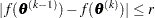
The same formula is used for the NMSIMP technique, but is defined as the vertex with the lowest function value, and is defined as the vertex with the highest function value in the simplex. The default value is . The optional integer value specifies the number of successive iterations for which the criterion must be satisfied before the process can be terminated.

specifies an absolute gradient convergence criterion. Termination requires the maximum absolute gradient element to be small:

This criterion is not used by the NMSIMP technique. The default value is E5. The optional integer value specifies the number of successive iterations for which the criterion must be satisfied before the process can be terminated.

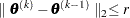
specifies an absolute parameter convergence criterion. For all techniques except NMSIMP, termination requires a small Euclidean distance between successive parameter vectors,

For the NMSIMP technique, termination requires either a small length of the vertices of a restart simplex,

or a small simplex size,

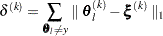
where the simplex size is defined as the L1 distance from the simplex vertex with the smallest function value to the other simplex points :

The default is E8 for the NMSIMP technique and otherwise. The optional integer value specifies the number of successive iterations for which the criterion must be satisfied before the process can terminate.

specifies the alpha level to be used in computing confidence limits. The default value is 0.05.

specifies an absolute singularity criterion for the computation of the inertia (number of positive, negative, and zero eigenvalues) of the Hessian and its projected forms. The default value is the square root of the smallest positive double-precision value.

specifies a multiplication factor for the estimated covariance matrix of the parameter estimates.

requests the approximate covariance matrix for the parameter estimates.

requests the approximate correlation matrix for the parameter estimates.

specifies a nonnegative threshold that determines whether the eigenvalues of a singular Hessian matrix are considered to be zero.

specifies that the initial step-size value for each line search (used by the QUANEW, CONGRA, or NEWRAP technique) cannot be larger than times the step-size value used in the former iteration. If you specify the DAMPSTEP option without factor , the default value is . The DAMPSTEP= option can prevent the line-search algorithm from repeatedly stepping into regions where some objective functions are difficult to compute or where they could lead to floating-point overflows during the computation of objective functions and their derivatives. The DAMPSTEP= option can save time-costly function calls that result in very small step sizes . For more details on setting the start values of each line search, see the section Restricting the Step Length.

specifies the input data set. Observations in this data set are used to compute the log likelihood function that you specify with PROC NLMIXED statements.

NOTE: If you are using a RANDOM statement, the input data set must be clustered according to the SUBJECT= variable. One easy way to accomplish this is to sort your data by the SUBJECT= variable prior to calling PROC NLMIXED. PROC NLMIXED does not sort the input data set for you.

specifies the degrees of freedom to be used in computing values and confidence limits. The default value is the number of subjects minus the number of random effects for random effects models, and the number of observations otherwise.

specifies that only the diagonal of the Hessian is used.

requests that a more comprehensive optimization be carried out if the default empirical Bayes optimization fails to converge.

specifies the step-shortening fraction to be used while computing empirical Bayes estimates of the random effects. The default value is 0.8.

specifies the objective function tolerance for determining the cessation of step-shortening while computing empirical Bayes estimates of the random effects. The default value is E8.

specifies the maximum number of Newton steps for computing empirical Bayes estimates of random effects. The default value is .

specifies the maximum number of step-shortenings for computing empirical Bayes estimates of random effects. The default value is .

specifies the convergence tolerance for empirical Bayes estimation. The default value is , where is the machine precision. This default value equals approximately E12 on most machines.

requests that a zero be used as starting values during empirical Bayes estimation. By default, the starting values are set equal to the estimates from the previous iteration (or zero for the first iteration).

requests the approximate covariance matrix for all expressions specified in ESTIMATE statements.

requests the approximate correlation matrix for all expressions specified in ESTIMATE statements.

requests the derivatives of all expressions specified in ESTIMATE statements with respect to each of the model parameters.

requests that the covariance matrix of the parameter estimates be computed as a likelihood-based empirical ("sandwich") estimator (White 1982). If is the objective function for the optimization and denotes the marginal log likelihood (see the section Modeling Assumptions and Notation for notation and further definitions) the empirical estimator is computed as

where is the second derivative matrix of and is the first derivative of the contribution to by the th subject. If you choose the EMPIRICAL option, this estimator of the covariance matrix of the parameter estimates replaces the model-based estimator in subsequent calculations. You can output the subject-specific gradients to a SAS data set with the SUBGRADIENT option in the PROC NLMIXED statement.

The EMPIRICAL option requires the presence of a RANDOM statement and is available for METHOD=GAUSS and METHOD=ISAMP only.

specifies a relative function convergence criterion. For all techniques except NMSIMP, termination requires a small relative change of the function value in successive iterations,

where FSIZE is defined by the FSIZE= option. The same formula is used for the NMSIMP technique, but is defined as the vertex with the lowest function value, and is defined as the vertex with the highest function value in the simplex. The default is , where FDIGITS is the value of the FDIGITS= option. The optional integer value specifies the number of successive iterations for which the criterion must be satisfied before the process can terminate.

specifies another function convergence criterion. For all techniques except NMSIMP, termination requires a small predicted reduction

of the objective function. The predicted reduction

is computed by approximating the objective function by the first two terms of the Taylor series and substituting the Newton step:

For the NMSIMP technique, termination requires a small standard deviation of the function values of the simplex vertices , ,

where . If there are boundary constraints active at , the mean and standard deviation are computed only for the unconstrained vertices. The default value is E6 for the NMSIMP technique and otherwise. The optional integer value specifies the number of successive iterations for which the criterion must be satisfied before the process can terminate.

specifies that all derivatives be computed using finite difference approximations. The following specifications are permitted:

FD

is equivalent to FD=100.

FD=CENTRAL

uses central differences.

FD=FORWARD

uses forward differences.

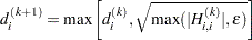
FD=

uses central differences for the initial and final evaluations of the gradient and for the Hessian. During iteration, start with forward differences and switch to a corresponding central-difference formula during the iteration process when one of the following two criteria is satisfied:

• The absolute maximum gradient element is less than or equal to times the ABSGCONV= threshold.

• The normalized predicted function reduction (see the GTOL option) is less than or equal to . The E6 ensures that the switch is done, even if you set the GTOL threshold to zero.

Note that the FD and FDHESSIAN options cannot apply at the same time. The FDHESSIAN option is ignored when only first-order derivatives are used. See the section Finite-Difference Approximations of Derivatives for more information.

specifies that second-order derivatives be computed using finite difference approximations based on evaluations of the gradients.

FDHESSIAN=FORWARD

uses forward differences.

FDHESSIAN=CENTRAL

uses central differences.

FDHESSIAN

uses forward differences for the Hessian except for the initial and final output.

Note that the FD and FDHESSIAN options cannot apply at the same time. See the section Finite-Difference Approximations of Derivatives for more information.

specifies the number of accurate digits in evaluations of the objective function. Fractional values such as FDIGITS=4.7 are allowed. The default value is , where is the machine precision. The value of is used to compute the interval size for the computation of finite-difference approximations of the derivatives of the objective function and for the default value of the FCONV= option.

displays a message for each statement in the model program as it is executed. This debugging option is very rarely needed and produces voluminous output.

specifies the FSIZE parameter of the relative function and relative gradient termination criteria. The default value is . For more details, see the FCONV= and GCONV= options.

specifies a dimension to determine the type of generalized inverse to use when the approximate covariance matrix of the parameter estimates is singular. The default value of is 60. See the section Covariance Matrix for more information.

specifies a relative gradient convergence criterion. For all techniques except CONGRA and NMSIMP, termination requires that the normalized predicted function reduction is small,

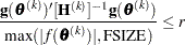
where FSIZE is defined by the FSIZE= option. For the CONGRA technique (where a reliable Hessian estimate is not available), the following criterion is used:

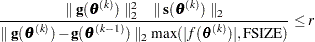
This criterion is not used by the NMSIMP technique.

The default value is E8. The optional integer value specifies the number of successive iterations for which the criterion must be satisfied before the process can terminate.

specifies the scaling version of the Hessian matrix used in NRRIDG, TRUREG, NEWRAP, or DBLDOG optimization.

If HS is not equal to 0, the first iteration and each restart iteration sets the diagonal scaling matrix :

where are the diagonal elements of the Hessian. In every other iteration, the diagonal scaling matrix is updated depending on the HS option:

HS=0

specifies that no scaling is done.

HS=1

specifies the Moré (1978) scaling update:

HS=2

specifies the Dennis, Gay, and Welsch (1981) scaling update:

HS=3

specifies that is reset in each iteration:

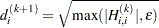
In each scaling update, is the relative machine precision. The default value is HS=0. Scaling of the Hessian can be time-consuming in the case where general linear constraints are active.

requests the display of the final Hessian matrix after optimization. If you also specify the START option, then the Hessian at the starting values is also printed.

specifies how the initial estimate of the approximate Hessian is defined for the quasi-Newton techniques QUANEW and DBLDOG. There are two alternatives:

• If you do not use the specification, the initial estimate of the approximate Hessian is set to the Hessian at .

• If you do use the specification, the initial estimate of the approximate Hessian is set to the multiple of the identity matrix, .

By default, if you do not specify the option INHESSIAN=, the initial estimate of the approximate Hessian is set to the multiple of the identity matrix , where the scalar is computed from the magnitude of the initial gradient.

reduces the length of the first trial step during the line search of the first iterations. For highly nonlinear objective functions, such as the EXP function, the default initial radius of the trust-region algorithm TRUREG or DBLDOG or the default step length of the line-search algorithms can result in arithmetic overflows. If this occurs, you should specify decreasing values of such as INSTEP=E1, INSTEP=E2, INSTEP=E4, and so on, until the iteration starts successfully.

• For trust-region algorithms (TRUREG, DBLDOG), the INSTEP= option specifies a factor for the initial radius of the trust region. The default initial trust-region radius is the length of the scaled gradient. This step corresponds to the default radius factor of .

• For line-search algorithms (NEWRAP, CONGRA, QUANEW), the INSTEP= option specifies an upper bound for the initial step length for the line search during the first five iterations. The default initial step length is .

• For the Nelder-Mead simplex algorithm, using TECH=NMSIMP, the INSTEP= option defines the size of the start simplex.

For more details, see the section Computational Problems.

requests a more complete iteration history, including the current values of the parameter estimates, their gradients, and additional optimization statistics. For further details, see the section Iterations.

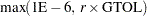
specifies a threshold for the Lagrange multiplier that determines whether an active inequality constraint remains active or can be deactivated. During minimization, an active inequality constraint can be deactivated only if its Lagrange multiplier is less than the threshold value . The default value is

where ABSGCONV is the value of the absolute gradient criterion, and is the maximum absolute element of the (projected) gradient or . (See the section Active Set Methods for a definition of .)

specifies the range for active and violated boundary constraints. The default value is E8. During the optimization process, the introduction of rounding errors can force PROC NLMIXED to increase the value of by a factor of . If this happens, it is indicated by a message displayed in the log.

specifies a criterion , used in the update of the QR decomposition, that determines whether an active constraint is linearly dependent on a set of other active constraints. The default value is E8. The larger becomes, the more the active constraints are recognized as being linearly dependent. If the value of is larger than , it is reset to .

specifies the line-search method for the CONGRA, QUANEW, and NEWRAP optimization techniques. See Fletcher (1987) for an introduction to line-search techniques. The value of can be . For CONGRA, QUANEW and NEWRAP, the default value is .

LIS=1

specifies a line-search method that needs the same number of function and gradient calls for cubic interpolation and cubic extrapolation; this method is similar to one used by the Harwell subroutine library.

LIS=2

specifies a line-search method that needs more function than gradient calls for quadratic and cubic interpolation and cubic extrapolation; this method is implemented as shown in Fletcher (1987) and can be modified to an exact line search by using the LSPRECISION= option.

LIS=3

specifies a line-search method that needs the same number of function and gradient calls for cubic interpolation and cubic extrapolation; this method is implemented as shown in Fletcher (1987) and can be modified to an exact line search by using the LSPRECISION= option.

LIS=4

specifies a line-search method that needs the same number of function and gradient calls for stepwise extrapolation and cubic interpolation.

LIS=5

specifies a line-search method that is a modified version of LIS=4.

LIS=6

specifies golden section line search (Polak 1971), which uses only function values for linear approximation.

LIS=7

specifies bisection line search (Polak 1971), which uses only function values for linear approximation.

LIS=8

specifies the Armijo line-search technique (Polak 1971), which uses only function values for linear approximation.

displays the model program and variable lists. The LIST option is a debugging feature and is not normally needed.

displays the derivative tables and the compiled program code. The LISTCODE option is a debugging feature and is not normally needed.

produces a report that lists, for each variable in the program, the variables that depend on it and on which it depends. The LISTDEP option is a debugging feature and is not normally needed.

displays a table of derivatives. This table lists each nonzero derivative computed for the problem. The LISTDER option is a debugging feature and is not normally needed.

writes periodic notes to the log that describe the current status of computations. It is designed for use with analyses requiring extensive CPU resources. The optional integer value specifies the desired level of reporting detail. The default is . Choosing adds information about the objective function values at the end of each iteration. The most detail is obtained with , which also reports the results of function evaluations within iterations.

specifies the degree of accuracy that should be obtained by the line-search algorithms LIS=2 and LIS=3. Usually an imprecise line search is inexpensive and successful. For more difficult optimization problems, a more precise and expensive line search might be necessary (Fletcher 1987). The second line-search method (which is the default for the NEWRAP, QUANEW, and CONGRA techniques) and the third line-search method approach exact line search for small LSPRECISION= values. If you have numerical problems, you should try to decrease the LSPRECISION= value to obtain a more precise line search. The default values are shown in the following table.

For more details, see Fletcher (1987).

specifies the maximum number of function calls in the optimization process. The default values are as follows:

• TRUREG, NRRIDG, NEWRAP: 125

• QUANEW, DBLDOG: 500

• CONGRA: 1000

• NMSIMP: 3000

Note that the optimization can terminate only after completing a full iteration. Therefore, the number of function calls that is actually performed can exceed the number that is specified by the MAXFUNC= option.

specifies the maximum number of iterations in the optimization process. The default values are as follows:

• TRUREG, NRRIDG, NEWRAP: 50

• QUANEW, DBLDOG: 200

• CONGRA: 400

• NMSIMP: 1000

These default values are also valid when is specified as a missing value.

specifies an upper bound for the step length of the line-search algorithms during the first iterations. By default, is the largest double-precision value and is the largest integer available. Setting this option can improve the speed of convergence for the CONGRA, QUANEW, and NEWRAP techniques.

specifies an upper limit of seconds of CPU time for the optimization process. The default value is the largest floating-point double representation of your computer. Note that the time specified by the MAXTIME= option is checked only once at the end of each iteration. Therefore, the actual running time can be much longer than that specified by the MAXTIME= option. The actual running time includes the rest of the time needed to finish the iteration and the time needed to generate the output of the results.

specifies the minimum number of iterations. The default value is 0. If you request more iterations than are actually needed for convergence to a stationary point, the optimization algorithms can behave strangely. For example, the effect of rounding errors can prevent the algorithm from continuing for the required number of iterations.

specifies a relative singularity criterion for the computation of the inertia (number of positive, negative, and zero eigenvalues) of the Hessian and its projected forms. The default value is E12 if you do not specify the SINGHESS= option; otherwise, the default value is . See the section Covariance Matrix for more information.

requests that the Gaussian quadrature be nonadaptive; that is, the quadrature points are centered at zero for each of the random effects and the current random-effects variance matrix is used as the scale matrix.

requests nonadaptive scaling for adaptive Gaussian quadrature; that is, the quadrature points are centered at the empirical Bayes estimates for the random effects, but the current random-effects variance matrix is used as the scale matrix. By default, the observed Hessian from the current empirical Bayes estimates is used as the scale matrix.

computes the function values of a grid of points in a ball of radius of about . If you specify the OPTCHECK option without factor , the default value is at the starting point and at the terminating point. If a point is found with a better function value than , then optimization is restarted at .

specifies an output data set containing the quadrature points used for numerical integration.

specifies the additive factor used to adaptively search for the number of quadrature points. For METHOD=GAUSS, the search sequence is 1, 3, 5, 7, 9, 11, 11 + , 11 + , ..., where the default value of is 10. For METHOD=ISAMP, the search sequence is 10, 10 + , 10 + , ..., where the default value of is 50.

specifies the maximum number of quadrature points permitted before the adaptive search is aborted. The default values are 31 for adaptive Gaussian quadrature, 61 for nonadaptive Gaussian quadrature, 160 for adaptive importance sampling, and 310 for nonadaptive importance sampling.

specifies the number of quadrature points to be used during evaluation of integrals. For METHOD=GAUSS, equals the number of points used in each dimension of the random effects, resulting in a total of points, where is the number of dimensions. For METHOD=ISAMP, specifies the total number of quadrature points regardless of the dimension of the random effects. By default, the number of quadrature points is selected adaptively, and this option disables the adaptive search.

specifies a multiplier for the scale matrix used during quadrature calculations. The default value is 1.0.

specifies the tolerance used to adaptively select the number of quadrature points. When the relative difference between two successive likelihood calculations is less than , then the search terminates and the lesser number of quadrature points is used during the subsequent optimization process. The default value is E4.

specifies that the QUANEW or CONGRA algorithm is restarted with a steepest descent/ascent search direction after, at most, iterations. Default values are as follows:

• CONGRA: UPDATE=PB: restart is performed automatically, is not used.

• CONGRA: UPDATEPB: , where is the number of parameters.

• QUANEW: is the largest integer available.

specifies the random number seed for METHOD=ISAMP. If you do not specify a seed, or if you specify a value less than or equal to zero, the seed is generated from reading the time of day from the computer clock. The value must be less than .

specifies the singularity criterion for Cholesky roots of the random-effects variance matrix and scale matrix for adaptive Gaussian quadrature. The default value is times the machine epsilon; this product is approximately E12 on most computers.

specifies the singularity criterion for the inversion of the Hessian matrix. The default value is E8. See the ASINGULAR, MSINGULAR=, and VSINGULAR= options for more information.

specifies the singularity criterion for inverting the variance matrix in the first-order method and the empirical Bayes Hessian matrix. The default value is times the machine epsilon; this product is approximately E12 on most computers.

specifies the singularity criterion below which statistical variances are considered to equal zero. The default value is times the machine epsilon; this product is approximately E12 on most computers.

requests that the gradient of the log likelihood at the starting values be displayed. If you also specify the HESS option, then the starting Hessian is displayed as well.

specifies a SAS data set to save in models with RANDOM statement the subject-specific gradients of the integrated, marginal log-likelihood with respect to all parameters. The sum of the subject-specific gradients equals the gradient reported in the "Parameter Estimates" table. The data set contains a variable identifying the subjects.

In models without RANDOM statement the SUBGRADIENT= data set contains the observation-wise gradient. The variable identifying the SUBJECT= is then replaced with the Observation. This observation counter includes observations not used in the analysis and is reset in each BY-group.

Saving disaggregated gradient information with the SUBGRADIENT= option requires METHOD=GAUSS or METHOD=ISAMP.

specifies the optimization technique. Valid values are as follows:

• CONGRA
  performs a conjugate-gradient optimization, which can be more precisely specified with the UPDATE= option and modified with the LINESEARCH= option. When you specify this option, UPDATE=PB by default.

• DBLDOG
  performs a version of double-dogleg optimization, which can be more precisely specified with the UPDATE= option. When you specify this option, UPDATE=DBFGS by default.

• NMSIMP
  performs a Nelder-Mead simplex optimization.

• NONE
  does not perform any optimization. This option can be used as follows:

  • to perform a grid search without optimization

  • to compute estimates and predictions that cannot be obtained efficiently with any of the optimization techniques

• NEWRAP
  performs a Newton-Raphson optimization combining a line-search algorithm with ridging. The line-search algorithm LIS=2 is the default method.

• NRRIDG
  performs a Newton-Raphson optimization with ridging.

• QUANEW
  performs a quasi-Newton optimization, which can be defined more precisely with the UPDATE= option and modified with the LINESEARCH= option. This is the default estimation method.

• TRUREG
  performs a trust region optimization.

displays the result of each operation in each statement in the model program as it is executed. This debugging option is very rarely needed, and it produces voluminous output.

specifies the update method for the quasi-Newton, double-dogleg, or conjugate-gradient optimization technique. Not every update method can be used with each optimizer. See the section Optimization Algorithms for more information.

Valid methods are as follows:

• BFGS
  performs the original Broyden, Fletcher, Goldfarb, and Shanno (BFGS) update of the inverse Hessian matrix.

• DBFGS
  performs the dual BFGS update of the Cholesky factor of the Hessian matrix. This is the default update method.

• DDFP
  performs the dual Davidon, Fletcher, and Powell (DFP) update of the Cholesky factor of the Hessian matrix.

• DFP
  performs the original DFP update of the inverse Hessian matrix.

• PB
  performs the automatic restart update method of Powell (1977) and Beale (1972).

• FR
  performs the Fletcher-Reeves update (Fletcher 1987).

• PR
  performs the Polak-Ribiere update (Fletcher 1987).

• CD
  performs a conjugate-descent update of Fletcher (1987).

specifies a relative singularity criterion for the computation of the inertia (number of positive, negative, and zero eigenvalues) of the Hessian and its projected forms. The default value is E8 if the SINGHESS= option is not specified, and it is the value of SINGHESS= option otherwise. See the section Covariance Matrix for more information.

specifies the relative parameter convergence criterion. For all techniques except NMSIMP, termination requires a small relative parameter change in subsequent iterations:

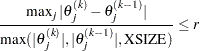
For the NMSIMP technique, the same formula is used, but is defined as the vertex with the lowest function value and is defined as the vertex with the highest function value in the simplex.

The default value is E8 for the NMSIMP technique and otherwise. The optional integer value specifies the number of successive iterations for which the criterion must be satisfied before the process can be terminated.

displays a cross-reference of the variables in the program showing where each variable is referenced or given a value. The XREF listing does not include derivative variables. This option is a debugging feature and is not normally needed.

specifies the XSIZE parameter of the relative parameter termination criterion. The default value is . For more details, see the XCONV= option.