| The NLMIXED Procedure |
| Modeling Assumptions and Notation |
PROC NLMIXED operates under the following general framework for nonlinear mixed models. Assume that you have an observed data vector  for each of
  subjects,
  . The are assumed to be independent across , but within-subject covariance is likely to exist because each of the elements of is measured on the same subject. As a statistical mechanism for modeling this within-subject covariance, assume that there exist latent random-effect vectors
  of small dimension (typically one or two) that are also independent across . Assume also that an appropriate model linking and exists, leading to the joint probability density function
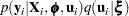 |
where  is a matrix of observed explanatory variables and
  and
and  are vectors of unknown parameters.
Let  and assume that it is of dimension
  . Then inferences about
  are based on the marginal likelihood function
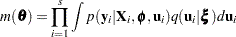 |
In particular, the function
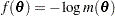 |
is minimized over numerically in order to estimate , and the inverse Hessian (second derivative) matrix at the estimates provides an approximate variance-covariance matrix for the estimate of . The function  is referred to both as the negative log likelihood function and as the objective function for optimization.
As an example of the preceding general framework, consider the nonlinear growth curve example in the section Getting Started: NLMIXED Procedure. Here, the conditional distribution  is normal with mean
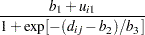 |
and variance  ; thus
  . Also,
  is a scalar and
  is normal with mean 0 and variance
  ; thus
  .
.
The following additional notation is also found in this chapter. The quantity  refers to the parameter vector at the
  th iteration, the vector
  refers to the gradient vector
  , and the matrix
  refers to the Hessian
  . Other symbols are used to denote various constants or option values.
Copyright © SAS Institute, Inc. All Rights Reserved.