The estimated covariance matrix of the parameter estimates is computed as the inverse Hessian matrix, and for unconstrained problems it should be positive definite. If the final parameter estimates are subjected to active linear inequality constraints, the formulas of the covariance matrices are modified similar to Gallant (1987) and Cramer (1986, p. 38) and additionally generalized for applications with singular matrices.

There are several steps available that enable you to tune the rank calculations of the covariance matrix.

1. You can use the ASINGULAR=, MSINGULAR=, and VSINGULAR= options to set three singularity criteria for the inversion of the Hessian matrix . The singularity criterion used for the inversion is

   where is the diagonal pivot of the matrix , and ASING, VSING, and MSING are the specified values of the ASINGULAR=, VSINGULAR=, and MSINGULAR= options, respectively. The default values are as follows:

   • ASING: the square root of the smallest positive double-precision value

   • MSING: E12 if you do not specify the SINGHESS= option and otherwise, where is the machine precision

   • VSING: E8 if you do not specify the SINGHESS= option and the value of SINGHESS otherwise

   Note that, in many cases, a normalized matrix is decomposed, and the singularity criteria are modified correspondingly.

2. If the matrix is found to be singular in the first step, a generalized inverse is computed. Depending on the G4= option, either a generalized inverse satisfying all four Moore-Penrose conditions is computed (a -inverse) or a generalized inverse satisfying only two Moore-Penrose conditions is computed (a -inverse, Pringle and Rayner, 1971). If the number of parameters of the application is less than or equal to G4=, a -inverse is computed; otherwise, only a -inverse is computed. The -inverse is computed by the (computationally very expensive but numerically stable) eigenvalue decomposition, and the -inverse is computed by Gauss transformation. The -inverse is computed using the eigenvalue decomposition , where is the orthogonal matrix of eigenvectors and is the diagonal matrix of eigenvalues, . The -inverse of is set to

   where the diagonal matrix is defined using the COVSING= option:

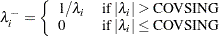
   If you do not specify the COVSING= option, the smallest eigenvalues are set to zero, where is the number of rank deficiencies found in the first step.

For optimization techniques that do not use second-order derivatives, the covariance matrix is computed using finite-difference approximations of the derivatives.