| The VARIOGRAM Procedure |
Example 95.3 Analysis without Surface Trend Removal
This example uses PROC VARIOGRAM without removing potential surface trends in a data set, in order to investigate a distinguished spatial direction in the data. In doing so, this example also serves as a guide to examine under which circumstances you might be able to bypass the effect of a trend on a semivariogram. Typically, though, for theoretical semivariogram estimations you follow the analysis presented in An Anisotropic Case Study with Surface Trend in the Data.
As explained in the section Details: VARIOGRAM Procedure, when you compute the empirical semivariance for data that contain underlying surface trends, the outcome is the pseudo-semivariance. Pseudo-semivariograms are not estimates of the theoretical semivariogram; hence, they do not provide any information about the spatial continuity of your SRF.
However, in the section Empirical Semivariograms and Surface Trends it is mentioned that you might still be able to perform a semivariogram analysis with potentially non-trend-free data, if you suspect that your measurements might be trend-free across one or more specific directions. The example demonstrates this approach.
Reconsider the ozone data presented at the beginning of An Anisotropic Case Study with Surface Trend in the Data. The spatial distribution of the data is shown in Figure 95.2.1, and the pairwise distance distribution for NHC=35 is illustrated in Figure 95.2.3. This exploratory analysis suggested a LAGDISTANCE=4 km, and Figure 95.2.2 indicated that for this LAGDISTANCE= you can consider a value of MAXLAGS=16.
Recall from the section Empirical Semivariograms and Surface Trends that you need to investigate the empirical semivariogram of the data in a few different directions, in order to identify a trend-free direction. If such a direction exists, then you can proceed with this special type of analysis. The following statements employ NDIRECTIONS=8 to examine eight directions:
   title 'Semivariogram Without Trend Removal Example';
   ods graphics on;
   proc variogram data=ozoneSet plot(only)=semivar;
      compute lagd=4 maxlag=16 ndirections=8 robust;
      coord xc=East yc=North;
      var Ozone;
   run;
By default, the range of  is divided into eight equally distanced angles:
  ,
,  ,
,  ,
,  ,
,  ,
,  ,
,  , and
, and  . The resulting empirical semivariograms for these angles are shown in Output 95.3.1.
 and
and 
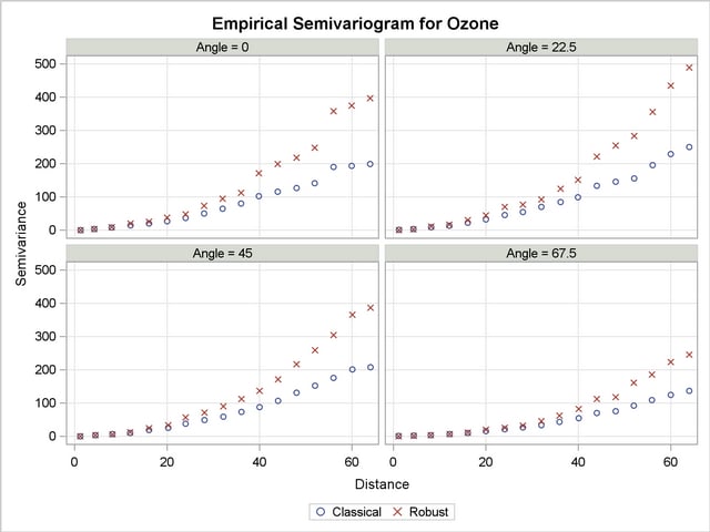
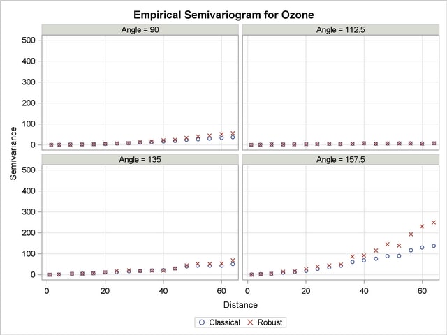
The figures in Output 95.3.1 suggest that in all directions there is an overall continuing increase with distance of the semivariance. As explained in the section Theoretical Semivariogram Models, this can be an indication of systematic trends in the data. However, in the direction of there is a clear indication that the increase rate, if any, is smaller than the corresponding rates across the rest of the directions. You then want to search whether there exists a trend-free direction in the neighborhood of this angle.
Run PROC VARIOGRAM again, specifying several directions within an interval of angles where you want to close in and suspect the existence of a trend-free direction. In the following step you use an ANGLETOL=15 , which is smaller than the default value of 22.5, as well as a BANDWIDTH=10 km. The smaller values help with minimization of the interference with neighboring directions, as discussed in the section Angle Classification.
The aforementioned considerations are addressed in the following statements:
   proc variogram data=ozoneSet plot(only)=semivar(cla);
      compute lagd=4 maxlag=16 robust;
      directions 100(15,10) 103(15,10)
                 106(15,10) 108(15,10)
                 110(15,10) 112(15,10)
                 115(15,10) 118(15,10);
      coord xc=East yc=North;
      var Ozone;
   run;
Your analysis has brought you to examine a narrow strip of angles within  and
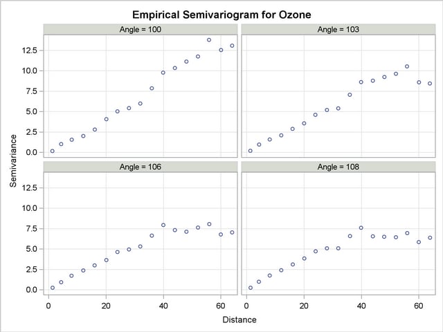
and  . The pseudo-semivariograms in Output 95.3.2 and Output 95.3.3 indicate that at the boundaries of this strip, the angles display increasing semivariance with distance. On the other hand, within this interval there are directions across which the semivariance is tentatively reaching a sill, and these are potential candidates to be trend-free directions.
 ,
,  ,
,  , and
, and 
 ,
,  ,
,  , and
, and 
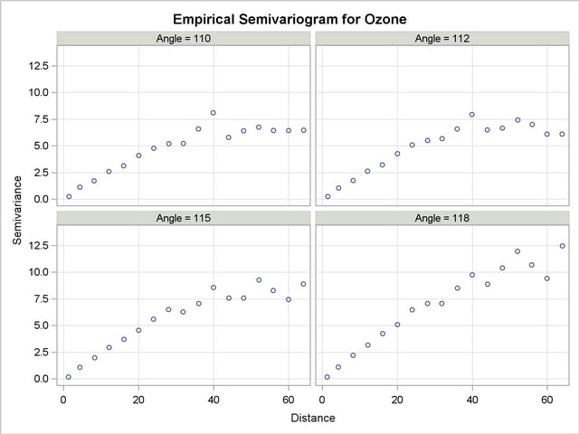
You could further investigate this angle spectrum in more detail. For example, you can monitor additional angles in between, or use a smaller LAGDISTANCE= and increased MAXLAGS= values to single out the most qualified candidate. For the purpose of this example, you can consider the direction  to very likely be the trend-free one you are looking for.
From a physical standpoint, it is also mentioned in the section Empirical Semivariograms and Surface Trends that you should expect the trend-free direction, if it exists, to be perpendicular to the direction of the maximum dip in the values of the ozone field. If you cross-examine the ozone data distribution in Output 95.2.1, the figure suggests that this direction exists and is slightly tilted clockwise with respect to the E–W axis. This direction emerges from the mild stratification of the ozone values in your data distribution. The ozone concentrations across it are similar when compared to surrounding directions, and as such, it has been identified as a trend-free direction.
Your next step is to obtain the empirical semivariogram in the suspected trend-free direction of , and to perform a theoretical model fit as shown in Theoretical Semivariogram Model Fitting and An Anisotropic Case Study with Surface Trend in the Data.
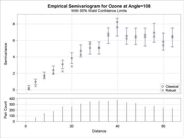
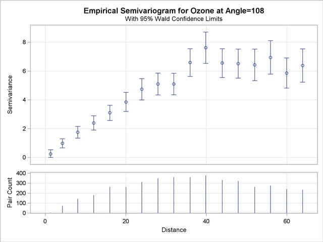
First, assume that you want to inspect the classical and robust empirical semivariograms in the selected direction, as well as a separate plot of the classical one and its confidence limits. Use the PLOT option as shown in the following statements to produce the two empirical semivariograms for your selected angle. The resulting plots are displayed in Output 95.3.4 and Output 95.3.5.
   proc variogram data=ozoneSet
                  plot(only)=(semivar semivar(cla));
      compute lagd=4 maxlag=16 robust cl;
      directions 108(15,10);
      coord xc=East yc=North;
      ods output SemivariogramTable=sv;
      var ozone;
   run;

Then, you create a vector of points on the Distance axis to provide enough theoretical model estimation locations for a smooth plot. Also, you combine this data set with the output of PROC VARIOGRAM to create the input data set for PROC NLIN. The statements you use are as follows:
   data pv;
      do Distance = 0 to 64 by 0.5;
         Semivariance = .;
         output;
      end;
   run;
   data sv; set sv pv; by Distance;
   run;
Finally, as in the previous examples, you employ PROC NLIN to fit a theoretical model to the empirical semivariogram shown in Output 95.3.5. Note that you have not omitted specifying the CL option earlier in the COMPUTE statement in PROC VARIOGRAM, so that you can provide PROC NLIN with semivariance variance information. The semivariance exhibits a slow, almost linear rise at short distances and seems to be reaching the sill fast, rather than asymptotically.
You can accommodate this behavior by using the following spherical model:
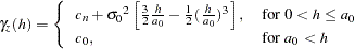 |
where  and
and  . PROC NLIN requires initial values for the model parameters. A reasonable initial choice for the sill value is about 7, and for the range
  km. Though there does not seem to be a nugget effect, you use an initial value
  and you initialize the partial sill by using
  . The following statements implement these considerations. Consequently, PROC SGPLOT is invoked to create the empirical and theoretical semivariogram plots.
   proc nlin data=sv;
      parms Nugget=0 Range=40 PartSill=7;
      if (Distance<Range)
         then y = Nugget + PartSill*(1.5*(Distance/Range) -
                                     0.5*(Distance/Range)**3);
         else y = Nugget + PartSill;
      model Semivariance = y;
      _weight_ = 1/SemivarianceStdErr/SemivarianceStdErr;
      output out=WLS p=WLSprediction;
   run;
   proc sgplot data=WLS;
      title "Empirical and Fitted Theoretical Semivariogram";
      xaxis label = "Distance" grid;
      yaxis label = "Semivariance" grid;
      scatter y=Semivariance x=Distance /
              markerattrs = GraphData1(symbol=circle)
              name='SemiVarClassical';
      series x=Distance y=WLSprediction /
             lineattrs = (thickness=2px color=black)
             name = 'SemivarPredWgh';
      discretelegend 'SemiVarClassical' 'SemivarPredWgh';
   run;

   ods graphics off;
PROC NLIN fits the requested model, for which the range, partial sill, and nugget effect estimates are shown in Figure 95.3.6. Clearly, there is an almost negligible nugget effect based on the weighted least squares PROC NLIN analysis. From the fitted values the estimate for the theoretical semivariogram sill is  . Figure 95.3.7 displays the fitted and empirical semivariograms in the selected direction .
| Parameter | Estimate | Approx Std Error |
Approximate 95% Confidence Limits |
|
|---|---|---|---|---|
| Nugget | 0.00991 | 0.1111 | -0.2284 | 0.2482 |
| Range | 47.0906 | 2.7872 | 41.1126 | 53.0685 |
| PartSill | 6.5461 | 0.2208 | 6.0725 | 7.0197 |
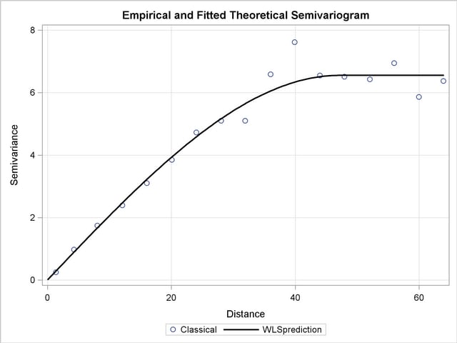
A comparative look at the empirical and fitted semivariograms in Output 95.3.7 and Output 95.2.8 suggests that the analysis of the trend-free ResidualOzone produces a different outcome from that of the original Ozone values. In fact, a more suitable comparison can be made between the semivariograms in the assumed trend-free direction of the current scenario, and the one shown in Output 95.2.6 in the nearly identical direction  . It might seem unreasonable that these two semivariograms are produced both in the same ozone study and in a narrow band of directions free of apparent surface trends, yet they bear no resemblance. However, the lack of similarity in these plots stems from operating on two different data sets where the outcome depends on the actual data values.
More specifically, in the eyes of semivariogram analysis the trend-free ozone set and the original ozone measurements are treated as different quantities. The process of detrending the original Ozone values is a transformation of these values into the trend-free ones of ResidualOzone. Any existing spatial correlation in the original data is not directly memorized into the transformed data, but is rather affected by the transformation features. In principle, the emerging data set has its own characteristics, as demonstrated in this example.
A final remark concerns the issue of isotropy. Based on the details presented in the section Empirical Semivariograms and Surface Trends, your knowledge of the spatial structure of the ozoneSet data set is limited to the selected trend-free direction you indicated in the present example. You can generalize this outcome for all spatial directions only if you consider the hypothesis of isotropy in the ozone field to be reasonable. Note that you cannot infer the assumption of anisotropy in the present example based on the analysis in the section Analysis with Surface Trend Removal. Again, the reason is that you currently use the observed Ozone values, whereas the ResidualOzone data in the previous example emerged from a transformation of the current data. Hence, you have essentially two data sets that do not necessarily share the same properties.
Copyright © 2009 by SAS Institute Inc., Cary, NC, USA. All rights reserved.