| The VARIOGRAM Procedure |
Analysis with Surface Trend Removal
You can use a SAS/STAT predictive modeling procedure to extract surface trends from your original data. If your goal is spatial prediction, you can continue processing the detrended data for the prediction tasks, and at the end you can reinstate the trend at the prediction locations to report your analysis results.
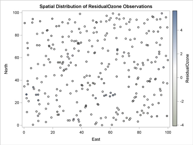
In general, the exact form of the trend is unknown, as discussed in the section Empirical Semivariograms and Surface Trends. In this case, the spatial distribution of the measurements shown in Figure 95.2.1 suggests that you can use a quadratic model to describe the surface trend like the one that follows:
 |
The following statements show how to invoke the GLM procedure for your ozone data, and how to extract the preceding trend from them:
   proc glm data=ozoneSet;
      model ozone = East East*East North North*North;
      output out=gmout predicted=pred residual=ResidualOzone;
   run;
Among other output, PROC GLM produces estimates for the parameters  in the preceding trend model. Output 95.2.4 shows the table with the parameter estimates. In this table, the coefficient
  corresponds to the intercept estimate, and the rest of the coefficients correspond to their matching variables; for example, the estimate in the line of "East*East" refers to
  in the preceding model. For more information about the syntax and the PROC GLM output, see
Chapter 39,
The GLM Procedure.
in the preceding model. For more information about the syntax and the PROC GLM output, see
Chapter 39,
The GLM Procedure.
| Parameter | Estimate | Standard Error | t Value | Pr > |t| |
|---|---|---|---|---|
| Intercept | 270.6798273 | 0.40595731 | 666.77 | <.0001 |
| East | 0.0065148 | 0.01360281 | 0.48 | 0.6323 |
| East*East | 0.0010726 | 0.00012987 | 8.26 | <.0001 |
| North | -0.0369159 | 0.01297491 | -2.85 | 0.0047 |
| North*North | 0.0035587 | 0.00012659 | 28.11 | <.0001 |
The detrending process leaves you with the GMOUT data set, which contains the ResidualOzone data residuals. You can run PROC VARIOGRAM again as follows, with the NOVARIOGRAM option to inspect the detrended residuals. Note that you ask only for the OBSERVATIONS plot, shown in Output 95.2.5.
   proc variogram data=gmout plots(only)=observ;
     compute novariogram nhc=35;
     coord xc=East yc=North;
     var ResidualOzone;
   run;
Before you proceed with the empirical semivariogram computation and model fitting, examine your data for anisotropy. This investigation is necessary to portray the spatial structure of your SRF accurately. If anisotropy exists, it will manifest itself as different ranges and/or sills for the empirical semivariograms in different directions.
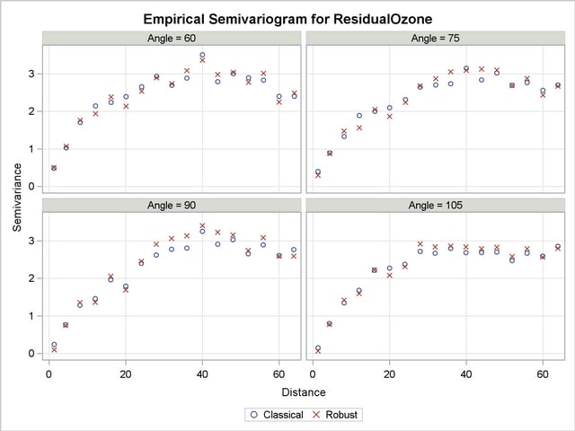
You want detail in your analysis, so you ask for the empirical semivariance in 12 directions by specifying NDIRECTIONS=12. Based on the NDIRECTIONS= option, empirical semivariograms are produced in increments of the base angle 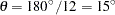 .
.
You also choose ANGLETOLERANCE=22.5 and BANDWIDTH=20. A different choice of values will produce different empirical semivariograms, because these options can regulate the number of pairs that are included in a class. You do not want these parameters to have values that are too small, so that you can allow for an adequate number of point pairs per class. On the other hand, the higher the values of these parameters, the more data pairs coming from closely neighboring directions will be included in each lag. In this case, there is a risk of losing information along the particular direction. This can be a side effect because you will incorporate data pairs from a broader spectrum of angles, and thus potentially amplify weaker anisotropy or weaken stronger anisotropy, as noted in the section Angle Classification. You can experiment with different ANGLETOLERANCE= and BANDWIDTH= values to reach this balance with your data, if necessary.
With the following statements you ask to display only the SEMIVAR plots in the specified number of directions. Multiple empirical semivariograms are placed by default in panels, as Output 95.2.6 shows. If you want an individual plot for each angle, then you need to further specify the plot option SEMIVAR(UNPACK).
   proc variogram data=gmout plot(only)=semivar;
      compute lagd=4 maxlag=16 ndir=12 atol=22.5 bandw=20 robust;
      coord xc=East yc=North;
      var ResidualOzone;
   run;
 and
and 
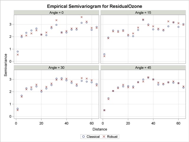
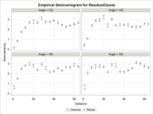
Note that in some of the directions, such as for  , the directional plots tend to exhibit a somewhat noisy structure. This behavior can be due to the pairs distribution across the particular direction. Specifically, based on the LAGDISTANCE= choice there might be insufficient pairs present in a class. Also, depending on the ANGLETOLERANCE= and BANDWIDTH= values, too many pairs might be considered from neighboring angles that potentially follow a modified structure. These are factors that can increase the variability in the semivariance estimate. A different explanation might lie in the existence of outliers in the data set; this aspect is further explored in A Box Plot of the Square Root Difference Cloud.
This behavior is relatively mild here and should not obstruct your goal to study anisotropy in your data. You can also perform individual computations in any direction. By doing so, you can fine-tune the computation parameters and attempt to obtain smoother estimates of the sample semivariance.
Further in this study, the directional plots in Output 95.2.6 suggest that during shifting from to  , the empirical semivariogram range increases. Beyond the angle , the range starts decreasing again until the whole circle is traversed at 180
 and small range values are encountered around the N–S direction at . Note that the sill seems to remain overall the same. This analysis suggests that there is anisotropy in the ozone concentrations, with the major axis oriented at about and the minor axis situated perpendicular to the major axis at .
The multidirectional analysis requires that for a given LAGDISTANCE= you also specify a MAXLAGS= value. Since the ozone correlation range might be unknown (as assumed here), you can apply the rule of thumb that suggests use of the half-extreme data distance in the direction of interest, as explained in the section Spatial Extent of the Empirical Semivariogram. Following the information displayed in Output 95.2.3, for different directions this distance varies between  and
and  km. In turn, the pairwise distances table in Output 95.2.2 indicates that within this range of distances you can specify MAXLAG= to be between 12 and 17 lags. In this example you specify MAXLAG=16.
At this point you are ready to continue with fitting theoretical semivariogram models to the empirical semivariogram in the selected directions of and . This process follows the exact steps shown in Theoretical Semivariogram Model Fitting. You apply weighted least squares fitting. In the following, PROC NLIN is used for the simultaneous theoretical semivariogram fitting in both directions of interest. By trying out different models, you see that an exponential one is suitable for your empirical data:
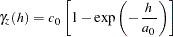 |
where  and
and  . First, you run PROC VARIOGRAM to create the necessary input information for PROC NLIN. The NLIN procedure needs information about the semivariance variance, which you obtain when you specify the CL option in the COMPUTE statement. You use the following statements:
   proc variogram data=gmout plot=none;
      compute lagd=4 maxlag=16 robust cl;
      directions 0(22.5,10) 90(22.5,10);
      coord xc=East yc=North;
      ods output SemivariogramTable=svg;
      var ResidualOzone;
   run;
You also request a vector of points throughout the Distance axis where PROC NLIN estimates the theoretical model values for the two selected directions. Note that essentially you need such a vector for each one of these directions. Then, the output of PROC VARIOGRAM is combined with the added Distance points into the PROC NLIN input data set, as shown in the following statements:
   data pv;
      do Angle = 0 to 90 by 90;
         do Distance = 0 to 64 by 0.5;
            Semivariance = .;
            output;
         end;
      end;
   run;
   data svg; set svg pv; by Angle Distance;
   run;
PROC NLIN requires initial values for the fitting parameters. For the direction, Output 95.2.6 suggests that a range  km (effective range
  km) and a partial sill
  can be used. Output 95.2.6 indicates that in the direction of , a range of
  km (effective range
  km) and a partial sill
  can be used. Both cases indicate that there is no significant nugget effect present. The nugget effect is initialized to the value
  . Note that you use one nugget effect value for all directions; that is, it is considered isotropic. The following statements implement these considerations, and PROC SGPLOT is eventually called to create the sample and theoretical semivariogram plots:
   proc nlin data=svg;
      parms Nugget=0 Range0=4   PartSill0=2.5
                     Range90=16 PartSill90=3;
      if (Angle=0) then
         y = Nugget + PartSill0*(1-exp(-Distance/Range0));
      else if (Angle=90) then
         y = Nugget + PartSill90*(1-exp(-Distance/Range90));
      model Semivariance = y;
      _weight_ = 1/SemivarianceStdErr/SemivarianceStdErr;
      output out=WLS p=WLSprediction;
   run;
   proc sgplot data=WLS;
      title "Empirical and Fitted Theoretical Semivariogram";
      xaxis label = "Distance" grid;
      yaxis label = "Semivariance" grid;
      scatter y=Semivariance x=Distance /
              name='SemiVarClassical'
              group=Angle;
      series x=Distance y=WLSprediction /
             lineattrs=(thickness=2px color=black)
             name='SemivarPredWgh'
             group=Angle;
      discretelegend 'SemiVarClassical' 'SemivarPredWgh';
   run;

   ods graphics off;
Output 95.2.7 shows the PROC NLIN estimates of the fitting parameters. From this table, you can easily compute the estimates for the sills in and , which are  and
and  , respectively. The fitted and empirical semivariograms are displayed in Output 95.2.8.
and
| Parameter | Estimate | Approx Std Error |
Approximate 95% Confidence Limits |
|
|---|---|---|---|---|
| Nugget | 0.0214 | 0.1517 | -0.2888 | 0.3316 |
| Range0 | 3.2073 | 1.1413 | 0.8730 | 5.5415 |
| PartSill0 | 2.5125 | 0.1677 | 2.1696 | 2.8554 |
| Range90 | 15.0962 | 2.7113 | 9.5510 | 20.6414 |
| PartSill90 | 2.8489 | 0.1740 | 2.4930 | 3.2048 |
and Directions
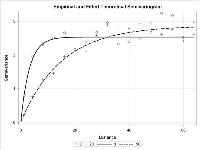
Conclusively, your semivariogram analysis on the detrended ozone data suggests that the ozone SRF exhibits anisotropy in the perpendicular directions of N–S () and E–W (). The sills in the two directions of anisotropy are similar in size, whereas the range in the major axis is about 4.5 times larger than the minor axis range.
Copyright © 2009 by SAS Institute Inc., Cary, NC, USA. All rights reserved.