Previous Page

|

Next Page

The VARIOGRAM Procedure

Empirical Semivariogram Computation

Using the values of LAGDISTANCE=7 and MAXLAGS=10 computed previously, rerun PROC VARIOGRAM without the NOVARIOGRAM option in order to compute the empirical semivariogram. You specify the CL option in the COMPUTE statement to calculate the 95% confidence limits for the classical semivariance. The section COMPUTE Statement describes how to use the ALPHA= option to specify a different confidence level.

Also, you can request a robust version of the semivariance with the ROBUST option in the COMPUTE statement. PROC VARIOGRAM produces a plot showing both the classical and the robust empirical semivariograms. See the details of the PLOT option to specify different instances of plots of the empirical semivariogram. In addition, ask for the autocorrelation Moran’s and Geary’s statistics under the assumption of randomization using binary weights. The following statements implement all of the preceding requests:

   proc variogram data=thick outv=outv;
      compute lagd=7 maxlag=10 cl robust
              autocorr(assum=random);
      coordinates xc=East yc=North;
      var Thick;
   run;
   
   ods graphics off;

Figure 95.6 displays the PROC VARIOGRAM output empirical semivariogram table for the preceding code.

Figure 95.6 Output Table for the Empirical Semivariogram Analysis

The VARIOGRAM Procedure

Dependent Variable: Thick

Empirical Semivariogram
Lag Class	Pair Count	Average Distance	Semivariance
			Robust	Classical	Standard Error	95% Confidence Limits
0	7	2.64	0.0284	0.0336	0.0179	0.000	0.0687
1	82	7.29	0.2098	0.3937	0.0615	0.273	0.5142
2	138	14.16	1.0079	1.1794	0.1420	0.901	1.4577
3	169	21.08	3.0183	2.7988	0.3045	2.202	3.3956
4	205	27.93	4.8107	4.6024	0.4546	3.711	5.4934
5	213	35.17	5.9904	5.9278	0.5744	4.802	7.0536
6	214	42.20	8.1040	7.5181	0.7268	6.094	8.9426
7	250	48.78	7.5326	7.2210	0.6459	5.955	8.4869
8	247	56.16	8.0662	7.1952	0.6475	5.926	8.4642
9	281	62.89	8.2792	6.8445	0.5774	5.713	7.9763
10	250	69.93	8.1440	6.3577	0.5686	5.243	7.4722

Figure 95.7 shows the output from the requested autocorrelation analysis. This includes the observed (computed) Moran’s and Geary’s coefficients, the expected value and standard deviation for each coefficient, the corresponding score, and the p-value in the Pr column. The low p-values suggest strong autocorrelation for both statistics types. Note that a two-sided p-value is reported, which is the probability that the observed coefficient lies farther away from on either side of the coefficient’s expected value—that is, lower than or higher than . The sign of for both Moran’s and Geary’s coefficients indicates positive autocorrelation in the Thick data values; see the section Interpretation for more details.

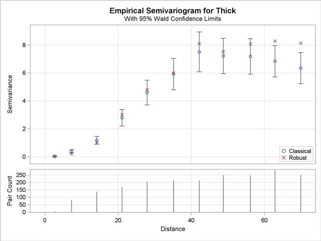
Figure 95.8 shows both the classical and robust empirical semivariograms. In addition, the plot features the approximate 95% confidence limits for the classical semivariance. The figure exhibits a typical behavior of the computed semivariance uncertainty, where in general the variance increases with distance from the origin at Distance=0.

The needle plot in the lower part of the Figure 95.8 provides the number of pairs that were used in the computation of the empirical semivariance for each lag class shown. Note that in general this is a pairwise distribution that is different from the distribution depicted in Figure 95.4. First, the number of pairs shown in the needle plot depends on the particular criteria you specify in the COMPUTE statement of PROC VARIOGRAM. Second, the distances shown for each lag on the Distance axis are not the midpoints of the lag classes as in the pairwise distances plot, but rather the average distance from the origin Distance=0 of all pairs in a given lag class.

Theoretical Semivariogram Model Fitting continues from this point to show how to choose a theoretical model for the thickness spatial dependence.

Figure 95.8 Classical and Robust Empirical Semivariograms for Coal Seam Thickness Data

Copyright © 2009 by SAS Institute Inc., Cary, NC, USA. All rights reserved.