| The TCALIS Procedure |
| The LISMOD Model and Submodels |
As a statistical model, the LISMOD modeling language is derived from the LISREL model proposed by Jöreskog and others (see Keesling 1972; Wiley 1973; Jöreskog 1973). But as a computer language, the LISMOD modeling language is quite different from the LISREL program. To maintain the consistence of specification syntax within the TCALIS procedure, the LISMOD modeling language departs from the original LISREL programming language. In addition, to make the programming a little easier, some terminological changes from LISREL are made in LISMOD.
For brevity, models specified by the LISMOD modeling language are called LISMOD models, although it is noted that you can also specify these so-called LISMOD models by other general modeling languages supported in PROC TCALIS.
The following descriptions of LISMOD models are basically the same as that of the original LISREL models. The main modifications are the names for the model matrices.
The LISMOD model is described by three component models. The first one is the structural equation model that describes the relationships among latent constructs or factors. The other two are measurement models that relate latent factors to manifest variables.
Structural Equation Model
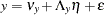
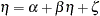
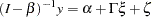
The structural equation model for latent factors is:
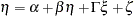 |
where:  is a random vector of
  endogenous latent factors
  is a random vector of
  exogenous latent factors
  is a random vector of errors
  is a vector of intercepts
  is a matrix of regression coefficients of variables on other variables
  is a matrix of regression coefficients of on
There are some assumptions in the structural equation model. To prevent a random variable in from regressing directly on itself, the diagonal elements of are assumed to be zeros. Also,  is assumed to be nonsingular, and is uncorrelated with .
The covariance matrix of is denoted by  and its expected value is a null vector. The covariance matrix of is denoted by
  and its expected value is denoted by
  .
.
Because variables in the structural equation model are not observed, to analyze the model these latent variables must somehow relate to the manifest variables. The measurement models, which will be discussed in the subsequent sections, provide such relations.
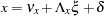
Measurement Model for 
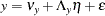 |
where:  is a random vector of
  manifest variables
  is a random vector of errors for
  is a vector of intercepts for
  is a matrix of regression coefficients of on
It is assumed that is uncorrelated with either or . The covariance matrix of is denoted by  and its expected value is the null vector.
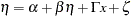
Measurement Model for 
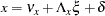 |
where:  is a random vector of
  manifest variables
  is a random vector of errors for
  is a vector of intercepts for
  is a matrix of regression coefficients of on
It is assumed that is uncorrelated with , , or . The covariance matrix of is denoted by  and its expected value is a null vector.
Covariance and Mean Structures
Under the structural and measurement equations and the model assumptions, the covariance structures of the manifest variables  are expressed as:
 |
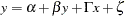
The mean structures of the manifest variables are expressed as:
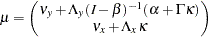 |
Model Matrices in the LISMOD Model
The parameters of the LISMOD model are elements in the model matrices, which are summarized as follows:
Matrix |
Name |
Description |
Dimensions |
Row Variables |
Column Variables |
|---|---|---|---|---|---|
|
_ALPHA_ |
intercepts for |
|
|
N/A |
|
_BETA_ |
effects of |
|
|
|
|
_GAMMA_ |
effects of |
|
|
|
|
_PSI_ |
error covariance matrix for |
|
|
|
|
_PHI_ |
covariance matrix for |
|
|
|
|
_KAPPA_ |
mean vector for |
|
|
N/A |
|
_NUY_ |
intercepts for |
|
|
N/A |
|
_LAMBDAY_ |
effects of |
|
|
|
|
_THETAY_ |
error covariance matrix for |
|
|
|
|
_NUX_ |
intercepts for |
|
|
N/A |
|
_LAMBDAX_ |
effects of |
|
|
|
|
_THETAX_ |
error covariance matrix for |
|
|
|


There are twelve model matrices in the LISMOD model. Not all of them are used in all situations. See the section LISMOD Submodels for details. In the table, each model matrix is given a name in the column Name, followed by a brief description of the parameters in the matrix, the dimensions, and the row and column variables being referred to. In the second column of the table, the LISMOD matrix names are used in the MATRIX statements when specifying the LISMOD model. In the last two columns of the table, following the row or column variables are the variable list (for example, ETAVAR=, YVAR=, and so on) in parentheses. These lists are used in the LISMOD statement for defining variables.
Specification of the LISMOD Model
The LISMOD specification is characterized by two tasks. The first task is to define the variables in the model. The second task is to specify the parameters in the LISMOD model matrices.
Specifying Variables
The first task is accomplished in the LISMOD statement. In the LISMOD statement, you define the lists of variables of interest: YVAR=, XVAR=, ETAVAR=, and XIVAR= lists, respectively for the -variables, -variables, -variables, and the -variables. While you provide the names of variables in these lists, you also define implicitly the numbers of four types of variables: , , , and . The variables on the YVAR= and XVAR= lists are manifest variables and therefore must be present in the analyzed data set. The variables on the ETAVAR= and XIVAR= lists are latent factors, the names of which are assigned by the researcher to represent their roles in the substantive theory. Once these lists are defined, the dimensions of the model matrices are also defined by the number of variables on various lists. In addition, the variable orders on the lists are referred to by the row and column variables of the model matrices.
Specifying Parameters in Model Matrices
The second task is accomplished by the MATRIX statements. In each MATRIX statement, you specify the model matrix by using the matrix names described in the previous table. Then you specify the parameters (free or fixed) in the locations of the model matrix. You can use as many MATRIX statements as needed for defining your model. But each model matrix can only be specified in one MATRIX statement and each MATRIX statement is used for specifying one model matrix.
An Example
In the section LISMOD Model, the LISMOD modeling language is used to specify the model described in the section A Structural Equation Example. In the LISMOD statement, you define four lists of variables, as shown in the following statement:
   lismod
      yvar  = Anomie67 Powerless67 Anomie71 Powerless71,
      xvar  = Education SEI,
      etav  = Alien67 Alien71,
      xivar = SES;
Endogenous latent factors are specified in the ETAVAR= list. Exogenous latent factors are specified in the XIVAR= list. In this case, Alien67 and Alien71 are the -variables, and SES is the only -variable in the model. Manifest variables that are indicators of endogenous latent factors in are specified in the YVAR= list. In this case, they are the Anomie and Powerless variables, measured in two different time points. Manifest variables that are indicators of exogenous latent factors in are specified in the XVAR= list. In this case, they are the Education and the SEI variables. Implicitly, the dimensions of the model matrices are defined by these lists already; that is,  ,
,  ,
,  , and
, and  .
.
The MATRIX statements are used to specify parameters in the model matrices. For example, in the following statement you define the _LAMBDAX_ () matrix with two nonzero entries:
    matrix _LAMBDAX_ [1,1] = 1.0,
                     [2,1] = lambda;
The first parameter location is for [1,1], which is the effect of SES (the first variable in the XIVAR= list) on Education (the first element in the XVAR= list). A fixed value of  is specified there. The second parameter location is for [2,1], which is the effect of SES (the first variable in the XIVAR= list) on SEI (the second variable in the XVAR= list). A parameter named lambda without initial value is specified there.
Another example is shown as follows:
   matrix _THETAY_  [1,1] = theta1,
                    [2,2] = theta2,
                    [3,3] = theta1,
                    [4,4] = theta2,
                    [3,1] = theta5,
                    [4,2] = theta5;
In this MATRIX statement, the error variances and covariances (that is, the matrix) for the -variables are specified. The diagonal elements of the _THETAY_ matrix are specified by parameters theta1, theta2, theta1, and theta2, respectively, for the four -variables Anomie67, Powerless67, Anomie71, and Powerless71. By using the same parameter name theta1, the error variances for Anomie67 and Anomie71 are implicitly constrained. Similarly, the error variances for Powerless67 and Powerless71 are also implicitly constrained. Two more parameter locations are specified. The error covariance between Anomie67 and Anomie71 and the error covariance between Powerless67 and Powerless71 are both represented by the parameter theta5. Again, this is an implicit constraint on the covariances. All other unspecified elements in the _THETAY_ matrix are treated as fixed zeros.
In this example, no parameters are specified for matrices _ALPHA_, _KAPPA_, _NUY_, or _NUX_. Therefore, mean structures are not modeled.
LISMOD Submodels
It is not necessary to specify all four lists of variables in the LISMOD statement. When some lists are unspecified in the LISMOD statement, PROC TCALIS will analyze submodels derived logically from the specified lists of variables. For example, if only - and - variable lists are specified, the submodel being analyzed would be a multivariate regression model with manifest variables only. Not all combinations of lists will lead to meaningful submodels, however. To determine whether and how a submodel (which is formed by a certain combination of variable lists) can be analyzed, the following three principles in the LISMOD modeling language are applied:
Submodels with at least one of the YVAR= and XVAR= lists are required.
Submodels that have an ETAVAR= list but no YVAR= list cannot be analyzed.
When a submodel has a YVAR= (an XVAR=) list but without an ETAVAR= (a XIVAR=) list, it is assumed that the set of
-variables (-variables) is equivalent to the -variables (-variables). Hereafter, this principle is referred to as an equivalence interpretation.
Apparently, the third principle is the same as the situation where the latent factors (or ) are perfectly measured by the manifest variables (or ). That is, in such a perfect measurement model, () is an identity matrix and () and () are both null. This can be referred to as a perfect measurement interpretation. However, the equivalence interpretation stated in the last principle presumes that there are actually no measurement equations at all. This is important because under the equivalence interpretation, matrices (), () and () are non-existent rather than fixed quantities, which is assumed under the perfect measurement interpretation. Hence, the -variables are treated as exogenous variables with the equivalence interpretation, but they are still treated as endogenous with the perfect measurement interpretation. Ultimately, whether -variables are treated as exogenous or endogenous will affect the default or automatic parameterization. See the section Default Parameters in the LISMOD Model for more details.
By using these three principles, the models and submodels that PROC TCALIS analyzes are summarized in the following table, followed by detailed descriptions of these models and submodels.
Presence of Lists |
Description |
Model Equations |
Non-fixed Model Matrices |
|
|---|---|---|---|---|
Presence of Both |
||||
1 |
YVAR=, ETAVAR=, |
full model |
|
|
XVAR=, XIVAR= |
|
|
||
|
|
|||
2 |
YVAR=, |
full model with |
|
|
XVAR=, XIVAR= |
|
|
|
|
3 |
YVAR=, ETAVAR=, |
full model with |
|
|
XVAR= |
|
|
|
|
4 |
YVAR=, |
regression |
|
|
XVAR= |
( |
|
||
( |
||||
Presence of |
||||
5 |
XVAR=, XIVAR= |
factor model |
|
|
for |
||||
6 |
XVAR= |
|
|
|
( |
||||
Presence of |
||||
7 |
YVAR=, ETAVAR= |
factor model |
|
|
for |
|
|
||
8 |
YVAR= |
|
|
|
( |
|
|||
9 |
YVAR=, ETAVAR=, |
second-order |
|
|
XIVAR= |
factor model |
|
|
|
10 |
YVAR=, |
factor model |
|
|
XIVAR= |
( |
|
||


 , or
, or 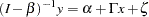
 , or
, or 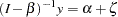
Models 1, 2, 3, and 4 — Presence of Both and Variables
Submodels 1, 2, 3, and 4 are characterized by the presence of both - and - variables in the model. Model 1 is in fact the full model with the presence of all four types of variables. All twelve model matrices are parameter matrices in this model.
Depending on the absence of the latent factor lists, manifest variables can replace the role of the latent factors in models 2–4. For example, the absence of the ETAVAR= list in model 2 means is equivalent to ( ). Consequently, you cannot, nor do you need to, use the MATRIX statement to specify parameters in the _LAMBDAY_, _THETAY_, or _NUY_ matrices under this model. Similarly, because is equivalent to (
 ) in model 3, you cannot, nor do you need to, use the MATRIX statement to specify the parameters in the _LAMBDAX_, _THETAX_, or _NUX_ matrices. In model 4, is equivalent to () and is equivalent to (). None of the six model matrices in the measurement equations are defined in the model. Matrices in which you can specify parameters by using the MATRIX statement are listed in the last column of the table.
Describing model 4 as a regression model is a simplification. Because can regress on itself in the model equation, the regression description is not totally accurate for model 4. Nonetheless, if is a null matrix, the equation describes a multivariate regression model with outcome variables and predictor variables . This model is the TYPE 2A model in LISREL VI (Jöreskog and Sörbom, 1985).
You should also be aware of the changes in meaning of the model matrices when there is an equivalence between latent factors and manifest variables. For example, in model 4 the and are now the covariance matrix and mean vector, respectively, of manifest variables , while in model 1 (the complete model) these matrices are of the latent factors .
Models 5 and 6 — Presence of Variables and Absence of Variables
Models 5 and 6 are characterized by the presence of the -variables and the absence of -variables.
Model 5 is simply a factor model for measured variables , with representing the factor loading matrix, the error covariance matrix, and the factor covariance matrix. If mean structures are modeled, represents the factor means and is the intercept vector. This is the TYPE 1 submodel in LISREL VI (Jöreskog and Sörbom, 1985).
Model 6 is a special case where there is no model equation. You specify the mean and covariance structures (in and , respectively) for the manifest variables directly. The -variables are treated as exogenous variables in this case. Because this submodel uses direct mean and covariance structures for measured variables, it can also be handled more easily by the MSTRUCT modeling language. See the MSTRUCT statement and the section The MSTRUCT Model for more details.
Note that because -variables cannot exist in the absence of -variables (see one of the three aforementioned principles in deriving submodels), adding the ETAVAR= list alone to these two submodels does not generate new submodels that can be analyzed by PROC TCALIS.
Models 7, 8 ,9 and 10—Presence of Variables and Absence of Variables
Models 7–10 are characterized by the presence of the -variables and the absence of -variables.
Model 7 is a factor model for -variables (TYPE 3B submodel in LISREL VI). It is similar to model 5, but with regressions among latent factors allowed. When is null, model 7 functions the same as model 5. It becomes a factor model for -variables, with representing the factor loading matrix, the error covariance matrix, the factor covariance matrix, the factor means, and the intercept vector.
Model 8 (TYPE 2B submodel in LISREL VI) is a model for studying the mean and covariance structures of -variables, with regression among -variables allowed. When is null, the mean structures of are specified in and the covariance structures are specified in . This is similar to model 6. However, there is an important distinction. In model 6, the variables are treated as exogenous (no model equation at all). But the -variables are treated as endogenous in model 8 (with or without  ). Consequently, the default parameterization would be different for these two submodels. See the section Default Parameters in the LISMOD Model for details about the default parameterization.
Model 9 represents a modified version of second-order factor model for . It would be a standard second-order factor model when is null. This is the TYPE 3A submodel in LISREL VI. With being null, represents the first-order factors and represents the second-order factors. The first- and second- order factor loading matrices are and , respectively.
Model 10 is another form of factor model when is null, with factors represented by and manifest variables represented by . However, if is indeed a null matrix in applications, you might want to use model 5, in which the factor model specification is more direct and intuitive.
Default Parameters in the LISMOD Model
When a model matrix is defined in a LISMOD model (or submodel), you can specify fixed values or parameters for the elements in the matrix. See the MATRIX statement for the syntax of specification. All other unspecified elements in the model matrices will be set by default. There are two types of default parameters: one is automatic free parameters; the other is fixed zeros.
Automatic Free Parameters
Automatic additions of free parameters are done to ensure the model is properly parameterized. Each automatic parameters is prefixed with _Add and appended with an unique integer. The following rules are used to add parameters in the LISMOD model matrices:
_THETAX_, _THETAY_, _PSI_, and _PHI_ matrices: If a matrix in this group is defined in a LISMOD submodel or full model, its diagonal elements are automatically represented by free parameters unless they are specified explicitly in the MATRIXstatements. This ensures that these covariance matrices will have nonzero variances.
_PHI_ matrix: For LISMOD submodels with XVAR= list specified but XIVAR= unspecified, all the off-diagonal elements of the _PHI_ are automatic free parameters. In this case, because
and are equivalent, its covariance matrix is the covariance matrix of exogenous manifest variables. Because exogenous covariances among manifest variables are not predicted as functions of any other parameters in the LISMOD model, they should be saturated by free parameters in the model unless there are theoretical reasons not to do so (for example, when you are testing a fixed pattern of these covariances). Failure to treat covariances among mainfest variables as free parameters is equivalent to fixing these values to constants, which leads to an overly restrictive model. _KAPPA_ matrix: For LISMOD submodels with XVAR= list specified but XIVAR= unspecified, all the elements of the _KAPPA_ vector are automatic free parameters if the mean structures are fitted. The reason for this is the same as the previous rule for adding covariance parameters among exogenous manifest variables. Exogenous manifest variables serve as explanatory variables in your model, and their means are not predicted by relationships with other variables. Unless you are also testing hypothesized mean values for the exogenous manifest variables, in general you should allow these means to be free parameters in the LISMOD model.
These three rules for automatic free parameters are in line with the treatments in the LINEQS, RAM, and PATH models. See, for example, the section Default Parameters in the LINEQS Model and the section Rationale of the Default Parameters in the LINEQS Model for details about the treatments of automatic free parameters.
Default Fixed Zeros
Matrix elements that are unspecified and are not automatic free parameters will be fixed at zeros by default.
Note: This procedure is experimental.
Copyright © 2009 by SAS Institute Inc., Cary, NC, USA. All rights reserved.