|
|
Example 25.1 Path Analysis: Stability of Alienation
The following covariance matrix from Wheaton et al. (1977) has served to illustrate the performance of several implementations for the analysis of structural equation models. Two different models have been analyzed by an early implementation of LISREL and are mentioned in Jöreskog (1978). You can also find a more detailed discussion of these models in the LISREL VI manual (Jöreskog and Sörbom 1985).
A slightly modified model for this covariance matrix is included in the EQS 2.0 manual (Bentler 1985, p. 28). The path diagram of this model is displayed in Figure 25.1. The same model is reanalyzed here by PROC CALIS. However, for the analysis with the EQS implementation, the last variable (V6) is rescaled by a factor of 0.1 to make the matrix less ill-conditioned. Since the Levenberg-Marquardt or Newton-Raphson optimization technique is used with PROC CALIS, rescaling the data matrix is not necessary and, therefore, is not done here. The results reported here reflect the estimates based on the original covariance matrix.
The DATA step and the CALIS model specification are shown as follows:
   data Wheaton(TYPE=COV);
   title "Stability of Alienation";
   title2 "Data Matrix of WHEATON, MUTHEN, ALWIN & SUMMERS (1977)";
      _type_ = 'cov'; input _name_ $ v1-v6;
      label v1='Anomie (1967)' v2='Anomie (1971)' v3='Education'
            v4='Powerlessness (1967)' v5='Powerlessness (1971)'
            v6='Occupational Status Index';
      datalines;
   v1   11.834     .        .        .       .        .
   v2    6.947    9.364     .        .       .        .
   v3    6.819    5.091   12.532     .       .        .
   v4    4.783    5.028    7.495    9.986    .        .
   v5   -3.839   -3.889   -3.841   -3.625   9.610     .
   v6  -21.899  -18.831  -21.748  -18.775  35.522  450.288
   ;
   ods graphics on;

   proc calis cov data=Wheaton tech=nr edf=931 pall plots=residuals;
      lineqs
         v1 =         f1                  + e1,
         v2 =    .833 f1                  + e2,
         v3 =         f2                  + e3,
         v4 =    .833 f2                  + e4,
         v5 =         f3                  + e5,
         v6 = Lamb (.5) f3                + e6,
         f1 = Gam1(-.5) f3                + d1,
         f2 = Beta (.5) f1 + Gam2(-.5) f3 + d2;
      std
         e1-e6 = The1-The2 The1-The4 (6 * 3.),
         d1-d2 = Psi1-Psi2 (2 * 4.),
         f3    = Phi (6.) ;
      cov
         e1 e3 = The5 (.2),
         e4 e2 = The5 (.2);
   run;

   ods graphics off;
The COV option in the PROC CALIS statement requests the analysis of the covariance matrix. Without the COV option, the correlation matrix would be computed and analyzed. Since no METHOD= option has been used, maximum likelihood estimates are computed by default. The TECH=NR option requests the Newton-Raphson optimization method. The PALL option produces the almost complete set of displayed output, as displayed in Output 25.1.1 through Output 25.1.23. Note that, when you specify the PALL option, you can produce large amounts of output. The PALL option is used in this example to show how you can get a wide spectrum of useful information from PROC CALIS.
PROC CALIS can produce a high-quality residual histogram that is useful for showing the distribution of residuals. To request the residual histogram, you must first enable ODS Graphics by specifying the ods graphics on statement, as shown in the preceding code before the PROC CALIS statement. Then, the residual histogram is requested by the plots=residuals option in the PROC CALIS statement.
Output 25.1.1 displays the model specification in matrix terms, followed by the lists of endogenous and exogenous variables. Output 25.1.2 displays equations and initial parameter estimates. You can use these output to ensure that the desired model is being analyzed.
Output 25.1.1
Model and Variables
The CALIS Procedure
Covariance Structure Analysis: Pattern and Initial Values
| _SEL_ |
6 |
17 |
SELECTION |
|
| _BETA_ |
17 |
17 |
EQSBETA |
IMINUSINV |
| _GAMMA_ |
17 |
9 |
EQSGAMMA |
|
| _PHI_ |
9 |
9 |
SYMMETRIC |
|
| |
| f3 |
| e1 e2 e3 e4 e5 e6 d1 d2 |
Output 25.1.2
Initial Model Specifications
Manifest Variable Equations with Initial Estimates
| v1 |
= |
1.0000 |
|
f1 |
+ |
1.0000 |
|
e1 |
| v2 |
= |
0.8330 |
|
f1 |
+ |
1.0000 |
|
e2 |
| v3 |
= |
1.0000 |
|
f2 |
+ |
1.0000 |
|
e3 |
| v4 |
= |
0.8330 |
|
f2 |
+ |
1.0000 |
|
e4 |
| v5 |
= |
1.0000 |
|
f3 |
+ |
1.0000 |
|
e5 |
| v6 |
= |
0.5000 |
* |
f3 |
+ |
1.0000 |
|
e6 |
| |
|
|
|
Lamb |
|
|
|
|
Latent Variable Equations with Initial Estimates
| f1 |
= |
-0.5000 |
* |
f3 |
+ |
1.0000 |
|
d1 |
|
|
|
|
| |
|
|
|
Gam1 |
|
|
|
|
|
|
|
|
| f2 |
= |
0.5000 |
* |
f1 |
+ |
-0.5000 |
* |
f3 |
+ |
1.0000 |
|
d2 |
| |
|
|
|
Beta |
|
|
|
Gam2 |
|
|
|
|
| Phi |
6.00000 |
| The1 |
3.00000 |
| The2 |
3.00000 |
| The1 |
3.00000 |
| The2 |
3.00000 |
| The3 |
3.00000 |
| The4 |
3.00000 |
| Psi1 |
4.00000 |
| Psi2 |
4.00000 |
| The5 |
0.20000 |
| The5 |
0.20000 |
General modeling information, descriptive statistics, and the input covariance matrix are displayed in Output 25.1.3. Because the input data set contains only the covariance matrix, the means of the manifest variables are assumed to be zero. Note that this has no impact on the estimation, unless a mean structure model is being analyzed.
Output 25.1.3
Modeling Information, Simple Statistics, and Input Covariance Matrix
| Anomie (1967) |
0 |
3.44006 |
| Anomie (1971) |
0 |
3.06007 |
| Education |
0 |
3.54006 |
| Powerlessness (1967) |
0 |
3.16006 |
| Powerlessness (1971) |
0 |
3.10000 |
| Occupational Status Index |
0 |
21.21999 |
| Anomie (1967) |
11.83400000 |
6.94700000 |
6.81900000 |
4.78300000 |
-3.83900000 |
-21.8990000 |
| Anomie (1971) |
6.94700000 |
9.36400000 |
5.09100000 |
5.02800000 |
-3.88900000 |
-18.8310000 |
| Education |
6.81900000 |
5.09100000 |
12.53200000 |
7.49500000 |
-3.84100000 |
-21.7480000 |
| Powerlessness (1967) |
4.78300000 |
5.02800000 |
7.49500000 |
9.98600000 |
-3.62500000 |
-18.7750000 |
| Powerlessness (1971) |
-3.83900000 |
-3.88900000 |
-3.84100000 |
-3.62500000 |
9.61000000 |
35.5220000 |
| Occupational Status Index |
-21.89900000 |
-18.83100000 |
-21.74800000 |
-18.77500000 |
35.52200000 |
450.2880000 |
The 12 parameter estimates in the model and their respective locations in the parameter matrices are displayed in Output 25.1.4. Each of the parameters, The1, The2, and The5, is specified for two elements in the parameter matrix _PHI_.
Output 25.1.4
Initial Estimates
| Beta |
0.50000 |
Matrix Entry: _BETA_[8:7] |
| Lamb |
0.50000 |
Matrix Entry: _GAMMA_[6:1] |
| Gam1 |
-0.50000 |
Matrix Entry: _GAMMA_[7:1] |
| Gam2 |
-0.50000 |
Matrix Entry: _GAMMA_[8:1] |
| Phi |
6.00000 |
Matrix Entry: _PHI_[1:1] |
| The1 |
3.00000 |
Matrix Entry: _PHI_[2:2] _PHI_[4:4] |
| The2 |
3.00000 |
Matrix Entry: _PHI_[3:3] _PHI_[5:5] |
| The5 |
0.20000 |
Matrix Entry: _PHI_[4:2] _PHI_[5:3] |
| The3 |
3.00000 |
Matrix Entry: _PHI_[6:6] |
| The4 |
3.00000 |
Matrix Entry: _PHI_[7:7] |
| Psi1 |
4.00000 |
Matrix Entry: _PHI_[8:8] |
| Psi2 |
4.00000 |
Matrix Entry: _PHI_[9:9] |
PROC CALIS examines whether each element in the moment matrix is modeled by the parameters defined in the model. If an element is not structured by the model parameters, it is predetermined by its observed value. This occurs, for example, when there are exogenous manifest variables in the model. If present, the predetermined values of the elements are displayed. In the current example, the ‘.’ displayed for all elements in the predicted moment matrix (Output 25.1.5) indicates that there are no predetermined elements in the model.
Output 25.1.5
Predetermined Elements
| Anomie (1967) |
. |
. |
. |
. |
. |
. |
| Anomie (1971) |
. |
. |
. |
. |
. |
. |
| Education |
. |
. |
. |
. |
. |
. |
| Powerlessness (1967) |
. |
. |
. |
. |
. |
. |
| Powerlessness (1971) |
. |
. |
. |
. |
. |
. |
| Occupational Status Index |
. |
. |
. |
. |
. |
. |
Output 25.1.6 displays the optimization information. You can check this table to determine whether the convergence criterion is satisfied. PROC CALIS displays an error message when problematic solutions are encountered.
Output 25.1.6
Optimization
Newton-Raphson Ridge Optimization
Without Parameter Scaling
| 0 |
119.33282242 |
| 74.016932345 |
|
| |
0 |
2 |
0 |
|
0.82689 |
118.5 |
1.3507 |
0 |
0.0154 |
| |
0 |
3 |
0 |
|
0.09859 |
0.7283 |
0.2330 |
0 |
0.716 |
| |
0 |
4 |
0 |
|
0.01581 |
0.0828 |
0.00684 |
0 |
1.285 |
| |
0 |
5 |
0 |
|
0.01449 |
0.00132 |
0.000286 |
0 |
1.042 |
| |
0 |
6 |
0 |
|
0.01448 |
9.936E-7 |
0.000045 |
0 |
1.053 |
| |
0 |
7 |
0 |
|
0.01448 |
4.227E-9 |
1.685E-6 |
0 |
1.056 |
| 6 |
8 |
| 7 |
0 |
| 0.0144844811 |
1.6847829E-6 |
| 0 |
1.0563187228 |
| ABSGCONV convergence criterion satisfied. |
Next, the predicted model matrix is displayed in the Output 25.1.7, followed by a list of model test statistics or fit indices (Output 25.1.8). Depending on your modeling philosophy, some indices might be preferred to others. In this example, all indices and test statistics point to a good fit of the model.
Output 25.1.7
Predicted Model Matrix
| Anomie (1967) |
11.90390632 |
6.91059048 |
6.83016211 |
4.93499582 |
-4.16791157 |
-22.3768816 |
| Anomie (1971) |
6.91059048 |
9.35145064 |
4.93499582 |
5.01664889 |
-3.47187034 |
-18.6399424 |
| Education |
6.83016211 |
4.93499582 |
12.61574998 |
7.50355625 |
-4.06565606 |
-21.8278873 |
| Powerlessness (1967) |
4.93499582 |
5.01664889 |
7.50355625 |
9.84539112 |
-3.38669150 |
-18.1826302 |
| Powerlessness (1971) |
-4.16791157 |
-3.47187034 |
-4.06565606 |
-3.38669150 |
9.61000000 |
35.5219999 |
| Occupational Status Index |
-22.37688158 |
-18.63994236 |
-21.82788734 |
-18.18263015 |
35.52199986 |
450.2879993 |
Output 25.1.8
Fit Statistics
| 0.0145 |
| 0.9953 |
| 0.9890 |
| 0.2281 |
| 0.0150 |
| 0.5972 |
| 13.4851 |
| 9 |
| 0.1419 |
| 2131.4 |
| 15 |
| 0.0231 |
| . |
| 0.0470 |
| 0.0405 |
| . |
| 0.0556 |
| 0.9705 |
| 0.9979 |
| 13.2804 |
| -4.5149 |
| -57.0509 |
| -48.0509 |
| 0.9976 |
| 0.9965 |
| 0.9937 |
| 0.5962 |
| 1.0754 |
| 0.9895 |
| 0.9979 |
| 1170 |
PROC CALIS can perform a detailed residual analysis. Large residuals might indicate misspecification of the model. In Output 25.1.9, raw residuals are reported and ranked. Because of the differential scaling of the variables, it is usually more useful to examine the standardized residuals instead. In Output 25.1.10, for example, the table for the 10 largest asymptotically standardized residuals is displayed. The model performs the poorest concerning the variable v5 and its covariance with v2, v1, and v3. This might suggest a misspecification of the model equation for v5. However, because the model fit is quite good, such a possible misspecification is not a serious concern in the analysis.
Output 25.1.9
Raw Residuals and Ranking
| Anomie (1967) |
-.0699063150 |
0.0364095216 |
-.0111621061 |
-.1519958205 |
0.3289115712 |
0.4778815840 |
| Anomie (1971) |
0.0364095216 |
0.0125493646 |
0.1560041795 |
0.0113511059 |
-.4171296612 |
-.1910576405 |
| Education |
-.0111621061 |
0.1560041795 |
-.0837499788 |
-.0085562504 |
0.2246560598 |
0.0798873380 |
| Powerlessness (1967) |
-.1519958205 |
0.0113511059 |
-.0085562504 |
0.1406088766 |
-.2383085022 |
-.5923698474 |
| Powerlessness (1971) |
0.3289115712 |
-.4171296612 |
0.2246560598 |
-.2383085022 |
0.0000000000 |
0.0000000000 |
| Occupational Status Index |
0.4778815840 |
-.1910576405 |
0.0798873380 |
-.5923698474 |
0.0000000000 |
0.0000000000 |
| -0.59237 |
| 0.47788 |
| -0.41713 |
| 0.32891 |
| -0.23831 |
| 0.22466 |
| -0.19106 |
| 0.15600 |
| -0.15200 |
| 0.14061 |
Output 25.1.10
Asymptotically Standardized Residuals and Ranking
| Anomie (1967) |
-0.308548787 |
0.526654452 |
-0.056188826 |
-0.865070455 |
2.553366366 |
0.464866661 |
| Anomie (1971) |
0.526654452 |
0.054363484 |
0.876120855 |
0.057354415 |
-2.763708659 |
-0.170127806 |
| Education |
-0.056188826 |
0.876120855 |
-0.354347092 |
-0.121874301 |
1.697931678 |
0.070202664 |
| Powerlessness (1967) |
-0.865070455 |
0.057354415 |
-0.121874301 |
0.584930625 |
-1.557412695 |
-0.495982427 |
| Powerlessness (1971) |
2.553366366 |
-2.763708659 |
1.697931678 |
-1.557412695 |
0.000000000 |
0.000000000 |
| Occupational Status Index |
0.464866661 |
-0.170127806 |
0.070202664 |
-0.495982427 |
0.000000000 |
0.000000000 |
| -2.76371 |
| 2.55337 |
| 1.69793 |
| -1.55741 |
| 0.87612 |
| -0.86507 |
| 0.58493 |
| 0.52665 |
| -0.49598 |
| 0.46487 |
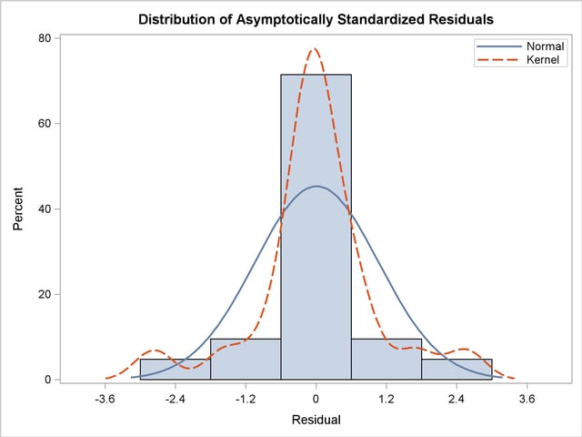
The histogram of the asymptotically standardized residuals is displayed in Output 25.1.11, which also shows the normal and kernel approximations. The residual distribution looks quite symmetrical. It shows a small to medium departure from the normal distribution, as evidenced by the discrepancies between the kernel and the normal distribution curves.
Output 25.1.11
Distribution of Asymptotically Standardized Residuals
Output 25.1.12 displays the equations and parameter estimates. Each parameter estimate is displayed with its standard error and the corresponding t ratio. As a general rule, a t ratio larger than 2 represents a statistically significant departure from 0. From these results, it is observed that both f1 (Alienation 1967) and f2 (Alienation 1971) are regressed negatively on f3 (Socioeconomic Status), and f1 has a positive effect on f2. The estimates and significance tests for the variance and covariance of the exogenous variables are also displayed.
Output 25.1.12
Equations and Parameter Estimates
Manifest Variable Equations with Estimates
| v1 |
= |
1.0000 |
|
f1 |
+ |
1.0000 |
|
e1 |
| v2 |
= |
0.8330 |
|
f1 |
+ |
1.0000 |
|
e2 |
| v3 |
= |
1.0000 |
|
f2 |
+ |
1.0000 |
|
e3 |
| v4 |
= |
0.8330 |
|
f2 |
+ |
1.0000 |
|
e4 |
| v5 |
= |
1.0000 |
|
f3 |
+ |
1.0000 |
|
e5 |
| v6 |
= |
5.3688 |
* |
f3 |
+ |
1.0000 |
|
e6 |
| Std Err |
|
0.4337 |
|
Lamb |
|
|
|
|
| t Value |
|
12.3788 |
|
|
|
|
|
|
Latent Variable Equations with Estimates
| f1 |
= |
-0.6299 |
* |
f3 |
+ |
1.0000 |
|
d1 |
|
|
|
|
| Std Err |
|
0.0563 |
|
Gam1 |
|
|
|
|
|
|
|
|
| t Value |
|
-11.1809 |
|
|
|
|
|
|
|
|
|
|
| f2 |
= |
0.5931 |
* |
f1 |
+ |
-0.2409 |
* |
f3 |
+ |
1.0000 |
|
d2 |
| Std Err |
|
0.0468 |
|
Beta |
|
0.0549 |
|
Gam2 |
|
|
|
|
| t Value |
|
12.6788 |
|
|
|
-4.3885 |
|
|
|
|
|
|
| Phi |
6.61632 |
0.63914 |
10.35 |
| The1 |
3.60788 |
0.20092 |
17.96 |
| The2 |
3.59493 |
0.16448 |
21.86 |
| The1 |
3.60788 |
0.20092 |
17.96 |
| The2 |
3.59493 |
0.16448 |
21.86 |
| The3 |
2.99368 |
0.49861 |
6.00 |
| The4 |
259.57580 |
18.31150 |
14.18 |
| Psi1 |
5.67047 |
0.42301 |
13.41 |
| Psi2 |
4.51480 |
0.33532 |
13.46 |
| The5 |
0.90580 |
0.12167 |
7.44 |
| The5 |
0.90580 |
0.12167 |
7.44 |
The measurement scale of variables is often arbitrary. Therefore, it can be useful to look at the standardized equations produced by PROC CALIS. Output 25.1.13 displays the standardized equations and predicted moments. From the standardized structural equations for f1 and f2, you can conclude that SES (f3) has a larger impact on earlier Alienation (f1) than on later Alienation (f3). The squared multiple correlation for each equation is also shown in Output 25.1.13. These correlations indicate the proportion of systematic variance in the equations. Finally, correlations among the exogenous variables are shown.
Output 25.1.13
Standardized Solutions
Manifest Variable Equations with Standardized Estimates
| v1 |
= |
0.8348 |
|
f1 |
+ |
0.5505 |
|
e1 |
| v2 |
= |
0.7846 |
|
f1 |
+ |
0.6200 |
|
e2 |
| v3 |
= |
0.8450 |
|
f2 |
+ |
0.5348 |
|
e3 |
| v4 |
= |
0.7968 |
|
f2 |
+ |
0.6043 |
|
e4 |
| v5 |
= |
0.8297 |
|
f3 |
+ |
0.5581 |
|
e5 |
| v6 |
= |
0.6508 |
* |
f3 |
+ |
0.7593 |
|
e6 |
| |
|
|
|
Lamb |
|
|
|
|
Latent Variable Equations with Standardized Estimates
| f1 |
= |
-0.5626 |
* |
f3 |
+ |
0.8268 |
|
d1 |
|
|
|
|
| |
|
|
|
Gam1 |
|
|
|
|
|
|
|
|
| f2 |
= |
0.5692 |
* |
f1 |
+ |
-0.2064 |
* |
f3 |
+ |
0.7080 |
|
d2 |
| |
|
|
|
Beta |
|
|
|
Gam2 |
|
|
|
|
| 3.60788 |
11.90391 |
0.6969 |
| 3.59493 |
9.35145 |
0.6156 |
| 3.60788 |
12.61575 |
0.7140 |
| 3.59493 |
9.84539 |
0.6349 |
| 2.99368 |
9.61000 |
0.6885 |
| 259.57580 |
450.28800 |
0.4235 |
| 5.67047 |
8.29603 |
0.3165 |
| 4.51480 |
9.00787 |
0.4988 |
| The5 |
0.25106 |
| The5 |
0.25197 |
The predicted covariances among the latent variables and between the observed and the latent variables are displayed in Output 25.1.14.
Output 25.1.14
Predicted Moments
| 8.296026985 |
5.924364730 |
-4.167911571 |
| 5.924364730 |
9.007870649 |
-4.065656060 |
| -4.167911571 |
-4.065656060 |
6.616317547 |
| 8.29602698 |
5.92436473 |
-4.16791157 |
| 6.91059048 |
4.93499582 |
-3.47187034 |
| 5.92436473 |
9.00787065 |
-4.06565606 |
| 4.93499582 |
7.50355625 |
-3.38669150 |
| -4.16791157 |
-4.06565606 |
6.61631755 |
| -22.37688158 |
-21.82788734 |
35.52199986 |
For interpreting the model, these predicted moments are not as useful as the main results shown previously. However, these predicted moments can be useful for further analysis. For example, they can be useful in constructing bootstrap "populations" for resampling. Another use of these moments is to compute the latent variable score regression coefficients. PROC CALIS computes these coefficients automatically, as shown in Output 25.1.15.
Output 25.1.15
Latent Variable Score Regression Coefficients
| Anomie (1967) |
0.4131113567 |
0.0482681051 |
-.0521264408 |
| Anomie (1971) |
0.3454029627 |
0.0400143300 |
-.0435560637 |
| Education |
0.0526632293 |
0.4306175653 |
-.0399927539 |
| Powerlessness (1967) |
0.0437036855 |
0.3600452776 |
-.0334000265 |
| Powerlessness (1971) |
-.0749215200 |
-.0639697183 |
0.5057060770 |
| Occupational Status Index |
-.0046390513 |
-.0039609288 |
0.0313127184 |
In Output 25.1.15, each latent variable is expressed as a linear combination of the observed variables. By computing these linear combinations for each individual, you can estimate the latent variable scores. See
Chapter 76,
The SCORE Procedure,
for more information about the creation of latent variable scores.
The total effects and indirect effects of the exogenous variables are displayed in Output 25.1.16. These results supplement to those shown in the linear equations in Output 25.1.12, which shows only the direct effects of predictor variables on outcome variables. Total, direct, and indirect effects have the following simple relationship:
| |
 |
|
|
To illustrate, consider the relationships between latent factor f3 and variables v1–v4. In the linear equations shown in Output 25.1.12, latent factor f3 does not have direct effects on variables v1–v4. This does not mean that f3 has no effects on these variables at all. As shown in the first table of Output 25.1.16, latent factor f3 indeed has nonzero total effects on all variables, including variables v1–v4. In the next table that shows indirect effects, latent factor f3, again, has nonzero indirect effects on variables v1–v4, and these effects are identical to the total effects. Because the sum of direct and indirect effects is the total effect, this means that the effects of f3 on v1–v4 are all indirect. Similar decomposition of effects can be made for other relationships. For example, while f1 has a total effect of  on v1, it has no indirect effect on v1. This means that all the effect of f1 on v1 is direct, which is also shown in an equation in Output 25.1.12. Finally, consider the effects of f3 on f2. In Output 25.1.16, latent factor f3 has nonzero total effect (
 ) and indirect effect (
 ) on f2, and these two effects are not identical. The difference of these two effects is the direct effect
  , as shown in an equation in Output 25.1.12.
Output 25.1.16
Total and Indirect Effects
| -0.629944307 |
1.000000000 |
0.000000000 |
| -0.524743608 |
0.833000000 |
0.000000000 |
| -0.614489258 |
0.593112208 |
1.000000000 |
| -0.511869552 |
0.494062469 |
0.833000000 |
| 1.000000000 |
0.000000000 |
0.000000000 |
| 5.368847492 |
0.000000000 |
0.000000000 |
| -0.629944307 |
0.000000000 |
0.000000000 |
| -0.614489258 |
0.593112208 |
0.000000000 |
| -.6299443069 |
0.0000000000 |
0 |
| -.5247436076 |
0.0000000000 |
0 |
| -.6144892580 |
0.5931122083 |
0 |
| -.5118695519 |
0.4940624695 |
0 |
| 0.0000000000 |
0.0000000000 |
0 |
| 0.0000000000 |
0.0000000000 |
0 |
| 0.0000000000 |
0.0000000000 |
0 |
| -.3736276589 |
0.0000000000 |
0 |
PROC CALIS can display Lagrange multiplier and Wald statistics for model modifications. Modification indices are displayed for each parameter matrix, as shown in Output 25.1.17 through Output 25.1.22. Only the Lagrange multiplier statistics have significance levels and approximate changes of values displayed. The significance level of the Wald statistic for a given parameter is the same as that shown in the equation output. An insignificant p-value for a Wald statistic means that the corresponding parameter can be dropped from the model without significantly worsening the fit of the model.
A significant p-value for a Lagrange multiplier test indicates that the model would achieve a better fit if the corresponding parameter were free. To aid in determining significant results, PROC CALIS displays the rank order of the 10 largest Lagrange multiplier statistics. For example, [E5:E2] in the _PHI_ matrix is associated with the largest Lagrange multiplier statistic; the associated p-value is  . This means that adding a parameter for the covariance between E5 and E2 will lead to a significantly better fit of the model. However, adding parameters indiscriminately can result in specification errors. An overfitted model might not perform well with future samples. As always, the decision to add parameters should be accompanied by consideration and knowledge of the application area.
Output 25.1.17
Lagrange Multiplier and Wald Tests for _PHI_
Output 25.1.18
Ranking of Lagrange Multipliers in _PHI_
| 7.36486 |
0.0067 |
| 5.80246 |
0.0160 |
| 3.39030 |
0.0656 |
| 3.39013 |
0.0656 |
| 1.59820 |
0.2062 |
| 1.41677 |
0.2339 |
| 1.20437 |
0.2724 |
| 1.20367 |
0.2726 |
| 1.18251 |
0.2768 |
| 1.18249 |
0.2768 |
Output 25.1.19
Lagrange Multiplier and Wald Tests for _GAMMA_
Output 25.1.20
Ranking of Lagrange Multipliers in _GAMMA_
| 3.39030 |
0.0656 |
| 3.39013 |
0.0656 |
| 0.57526 |
0.4482 |
| 0.57523 |
0.4482 |
Output 25.1.21
Lagrange Multiplier and Wald Tests for _BETA_
Output 25.1.22
Ranking of Lagrange Multipliers in _BETA_
| 8.64546 |
0.0033 |
| 5.88576 |
0.0153 |
| 5.40848 |
0.0200 |
| 5.40832 |
0.0200 |
| 2.71233 |
0.0996 |
| 2.14572 |
0.1430 |
| 1.61279 |
0.2041 |
| 1.61137 |
0.2043 |
| 1.43867 |
0.2304 |
| 1.15372 |
0.2828 |
When you specify equality constraints, PROC CALIS displays Lagrange multiplier tests for releasing the constraints, as shown in Output 25.1.23. In the current example, none of the three constraints achieve a p-value smaller than  . This means that releasing the constraints might not lead to a significantly better fit of the model. Therefore, all constraints are retained in the model.
Output 25.1.23
Tests for Equality Constraints
| 0.0293 |
-0.0308 |
0.02106 |
0.8846 |
| -0.1342 |
0.1388 |
0.69488 |
0.4045 |
| 0.2468 |
-0.1710 |
1.29124 |
0.2558 |
The current model is specified using the LINEQS, STD, and COV statements. As discussed in the section Getting Started: CALIS Procedure, you can also specify the same model by using other specification methods. In the following statements, equivalent COSAN and RAM specifications of the current model are shown. These two specifications would give essentially the same estimation results for the model specified using the LINEQS model statements.
   proc calis cov data=Wheaton tech=nr edf=931;
      Cosan J(9, Ide) * A(9, Gen, Imi) * P(9, Sym);
      Matrix A
              [ ,7] = 1. .833  5 * 0. Beta (.5) ,
              [ ,8] = 2 * 0.  1.  .833 ,
              [ ,9] = 4 * 0.  1.  Lamb Gam1-Gam2 (.5 2 * -.5);
      Matrix P
              [1,1] = The1-The2 The1-The4 (6 * 3.) ,
              [7,7] = Psi1-Psi2 Phi (2 * 4. 6.) ,
              [3,1] = The5 (.2) ,
              [4,2] = The5 (.2) ;
      Vnames J V1-V6 F1-F3 ,
             A = J ,
             P E1-E6 D1-D3 ;
   run;
   proc calis cov data=Wheaton tech=nr edf=931;
      Ram
         1   1  7  1.       ,
         1   2  7  .833     ,
         1   3  8  1.       ,
         1   4  8  .833     ,
         1   5  9  1.       ,
         1   6  9  .5    Lamb ,
         1   7  9  -.5   Gam1 ,
         1   8  7  .5    Beta ,
         1   8  9  -.5   Gam2 ,
         2   1  1  3.    The1 ,
         2   2  2  3.    The2 ,
         2   3  3  3.    The1 ,
         2   4  4  3.    The2 ,
         2   5  5  3.    The3 ,
         2   6  6  3.    The4 ,
         2   1  3  .2    The5 ,
         2   2  4  .2    The5 ,
         2   7  7  4.    Psi1 ,
         2   8  8  4.    Psi2 ,
         2   9  9  6.    Phi ;
      Vnames 1 F1-F3,
             2 E1-E6 D1-D3;
   run;
Copyright
© 2009 by SAS Institute Inc., Cary, NC, USA. All
rights reserved.